Let’s learn how to model time series data using some simple commands and tricks on Stata!

Hey Guys! What’s up? It’s been a while since my last post.. But now I am here to maintain the promise I made you. The hot topic will be how to model AR(), MA(), ARIMA and ARMAX(). As usual, I suggest you to check the theory behind the commands before we start.

Basically, we can operate in two way to model time series. The first is by hand, using the famous regress command. Let’s start by opening the dataset:

sysuse gnp96.dta

As you can see, this dataset is extremely poor because it’s made by just one series: the Real Gross National Product. In order to understand which kind of series are we facing let’s check its graph:

twoway (tsline ln_wpi)

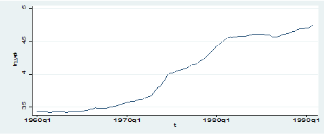
We are clearly dealing with a non-stationary time series with an upward trend so, if we want to implement a simple AR(1) model we know that we have to perform it on first-differenced series to obtain some sort of stationarity, as seen here.

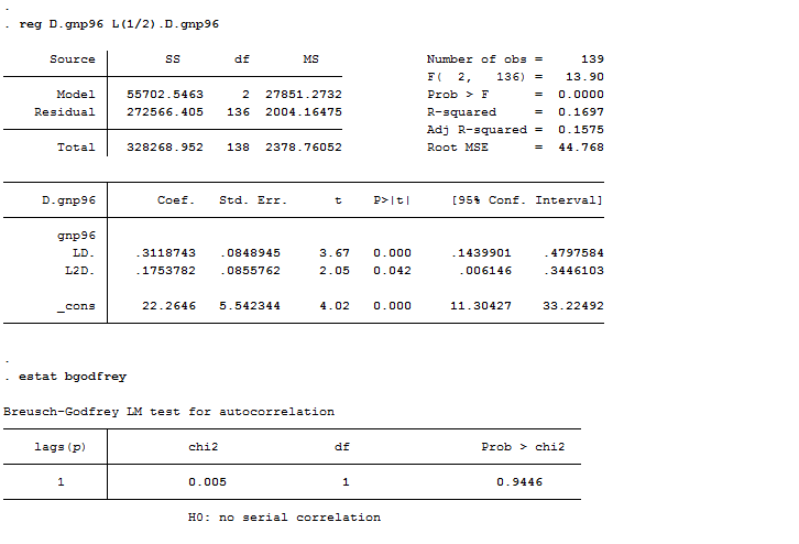
reg D.gnp96 L.D.gnp96

estat bgodfrey

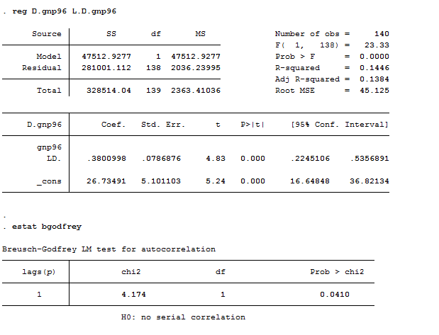
I estimated an AR(1) model on the differenced series that seems not to be the “best” choice, considering that errors are serially correlated. Then I performed an AR(2) model that behaves better.  L(1/2) means that Stata has to regress the first difference of gnp96 on its first and second lags.

reg D.gnp96 L(1/2).D.gnp96

estat bgodfrey

I could have also added the vce(robust) option to control for robust standard errors. Hypothesis test in this case works as usual:

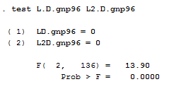
We can reject the null hypothesis that the coefficients are equal to zero jointly. Another useful option when you play manually with time series is the if tin(.) that restricts the sample to times in the specified range of dates, in this case from 1970 first quarter through 1990 fourth quarter.

regress D.gnp96 L.D.gnp96 if tin(1970q1,1990q4), vce(robust)

Another way to manually implement time series models is by using the Newey-West Heteroskedastic-and-Autocorrelation-Consistent Standard Errors. To use this command we need more than one series so let’s change our dataset:

use http://www.stata-press.com/data/imeus/ukrates, clear

If you don’t remember when we used these data, you are kindly invited to check it here.

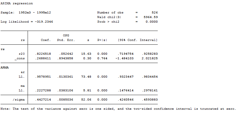
newey rs r20, lag(2)

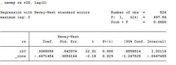
Regress the monthly change in the short rates rs (Bank’s of England’s monetary policy instrument) as a function of the prior month’s change in the long-term rate r20, assuming that the error term times each right-hand-side variable is autocorrelated for up to # periods of time.  (If # is 0, this is the same as regression with robust standard errors.)  A rule of thumb is to choose # = 0.75 * T^(1/3), rounded to an integer, where T is the number of observations used in the regression.  If there is strong serial correlation, # might be made more than this rule of thumb suggests, while if there is little serial correlation, # might be made less than this rule of thumb suggests.

ARIMA models

Stata created a useful command that computes every model automatically; you just need to know its components to use it at it best. Stata’s capabilities to estimate ARIMA or ‘Box–Jenkins’ models are thus implemented by the arima() command. These modeling tools include both the traditional ARIMA(p, d, q) framework as well as multiplicative seasonal ARIMA components for a univariate time series model. The arima command also implements ARMAX models: that is, regression equations with ARMA errors. In both the ARIMA and ARMAX contexts, the arima command implements dynamic forecasts, where successive forecasts are based on their own predecessors, rather than being one-step-ahead (static) forecasts. Let’s play! I will use directly ARMAX models to show you a bit of regressions.

Basic syntax for a regression model with ARMA disturbances:

arima rs r20, ar(1) ma(1)

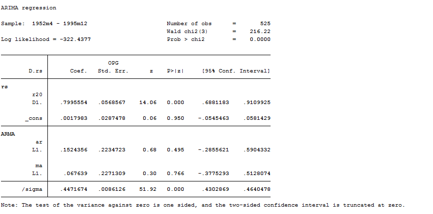
I just showed you this model for teaching reasons. We obviously know the series aren’t stationary so an ARMA model is not correct. We need to perform an ARIMA model that it could be either fitted by:

arima rs r20, arima(1,1,1)  or

arima D.rs D.r20, ar(1) ma(1)

The estimation sample runs through 1994m12.

Let’s now change the dataset and compute forecasts. We are going to use a big one:

use http://fmwww.bc.edu/cfb/data/usmacro1,clear

To illustrate forecasts, we fit an ARIMA(p,d,q) model to the US consumer price index (CPI):

arima cpi, arima(1, 1, 1) nolog

estimates store et1

Several prediction options are available after estimating an arima model. The default option, xb, predicts the actual dependent variable: so if D.cpi is the dependent variable, predictions are made for that variable. In contrast, the y option generates predictions of the original variable, in this case cpi. The mse option calculates the mean squared error of predictions, while yresiduals are computed in terms of the original variable.

We recall the estimates from the first model fitted, and calculate predictions for the actual dependent variable, ∆CPI:

estimates restore et1

predict double dcpihat, xb

tsline dcpihat, ti(“ARIMA(1,1,1) model of {&Delta}US CPI”) scheme(s2mono)

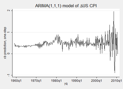
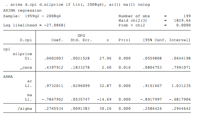
We can see that the predictions are becoming increasingly volatile in recent years. We now illustrate the estimation of an ARMAX model of ∆cpi as a function of ∆oilprice with ARMA(1, 1) errors. The estimation sample runs through 2008q4:

arima d.cpi d.oilprice if tin(, 2008q4), ar(1) ma(1) nolog

We can now use these data to compute static (one-period-ahead) ex ante forecasts and dynamic (multi-period-ahead) ex ante forecasts for 2009q1–2010q3. In specifying the dynamic forecast, the dynamic( ) option indicates the period in which references to y should first evaluate to the prediction of the model rather than historical values. In all prior periods, references to y are to the actual data.

predict double cpihat_s if tin(2006q1,), y

label var cpihat_s “static forecast”

predict double cpihat_d if tin(2006q1,), dynamic(tq(2008q4)) y

label var cpihat_d “dynamic forecast”

tw (tsline cpihat_s cpihat_d if !mi(cpihat_s)) (scatter cpi yq if !mi(cpihat_s), c(i)), scheme(s2mono) ti(“Static and dynamic ex ante forecasts of US CPI”) t2(“Forecast horizon: 2009q1-2010q3”) legend(rows(1))

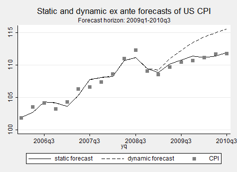
Once you can plot something like that you start feeling powerful. That’s the beauty of STATA!

We are forgetting that arima, as every other command, allows for postestimation commands of special interest. The ones you mainly use are:

estat acplot  // it estimates autocorrelations and autocovariances

estat aroots // It checks stability condition of estimates

estat ic // Displays AIC and BIC selection criterias

irf // Extremely importan ( I am not running into it today) It creates and analyzes Impulse Response Functions.

psdensity // to estimate the spectral density

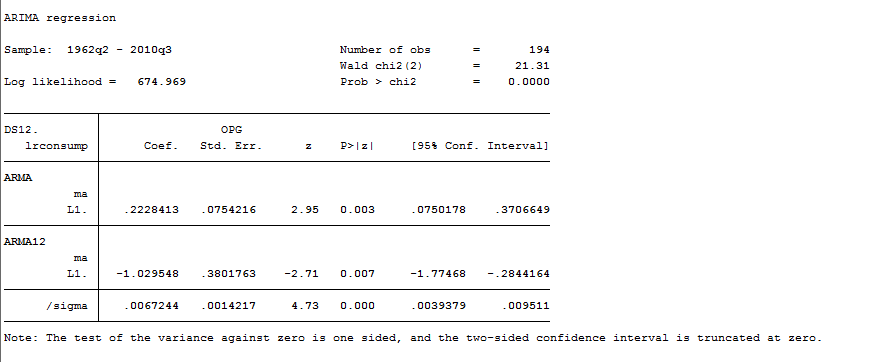
Many time series exhibit a periodic seasonal component, and a seasonal ARIMA model, often abbreviated SARIMA, can then be used. For example, monthly sales data for air conditioners have a strong seasonal component, with sales high in the summer months and low in the winter months. If a plot of the data suggests that the seasonal effect is proportional to the mean of the series, then the seasonal effect is probably multiplicative and a multiplicative SARIMA model may be appropriate. Box, Jenkins, and Reinsel (2008, sec. 9.3.1) suggest starting with a multiplicative SARIMA model with any data that exhibit seasonal patterns and then exploring non-multiplicative SARIMA models if the multiplicative models do not fit the data well. On the other hand, Chatfield (2004, 14) suggests that taking the logarithm of the series will make the seasonal effect additive, in which case an additive SARIMA model as fit in the previous example would be appropriate. In short, the analyst should probably try both additive and multiplicative SARIMA models to see which provides better fits and forecasts. Let’s try by using the logarithm of the real household consumption expenditures:

arima lrconsump,  arima(0,1,1) sarima(0,1,1,12) noconstant

Dynamic Multipliers and Cumulative Dynamic Multipliers

In order to explore this theme we are going to change dataset, again. We will need to use the data on growth provided by Stock and Watson in their book. You can download the file from:

http://www.learneconometrics.com/class/5263/2012/

Unfortunately, I cannot upload .dta files on my blog so I need to surf the web to find them. On the Data part, you can find a hyperlink “US Monthly macro data”. If you click on it, you will download the file we need. Once you installed it, open and explore it. If you estimate the effect of multiple lags of X on Y, then the estimated effects on Y are effects that occur after different amounts of time.  In order to compute ths model we need to prepare the data before:

generate time = m(1947m1) + _n-1

format t %tm

tsset time

generate L_ip = L1.ip

generate ip_growth = 100 * log(ip/L_ip)

summarize if tin(1952m1, 2009m12)

tsline oil

generate D_oil = D.oil

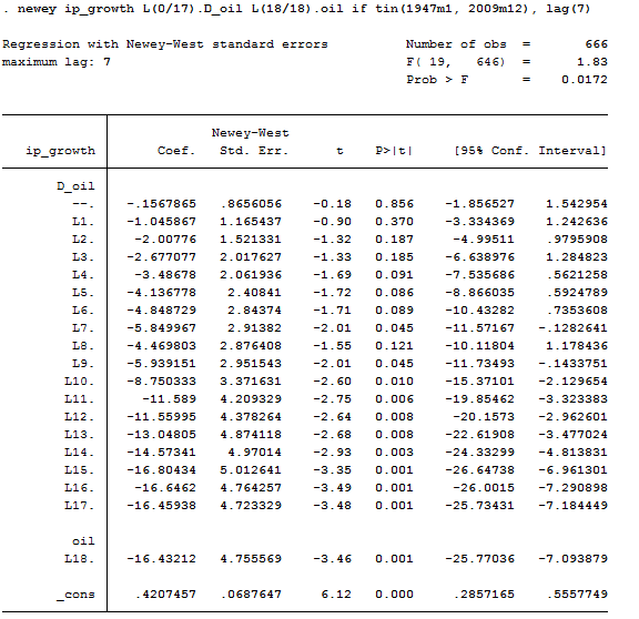
Here, the growth rate of industrial production (ipgrowth) is related to the percentage oil price increase or 0 if there was no oil price increase (oilshock) in 18 previous months.  This provides estimates of the effects of oil price shocks after 1 month, after 2 months, etc.

* non-cumulative effects

newey ip_growth L(0/18).oil if tin(1947m1, 2009m12), lag(7)

testparm L(0/18).oil

* cumulative effects

newey ip_growth L(0/17).D_oil L(18/18).oil if tin(1947m1, 2009m12), lag(7)

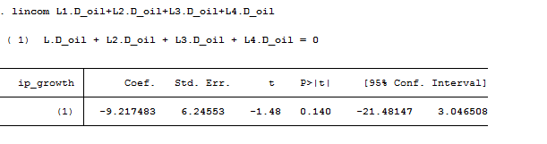
The cumulative effect after 4 months then could be found by:

lincom L1.D_oil+L2.D_oil+L3.D_oil+L4.D_oil

Confidence intervals and p-values are reported along with these results. You could draw by hand a graph of the estimated effects versus the time lag, along with 95% confidence intervals.  You could also draw by hand a graph of the estimated cumulative effects versus the time lag, along with 95% confidence intervals.  Making the same graphs in an automated fashion in Stata is a little more painstaking.

Ok guys. Let’s stop there for now. Soon we will go through multivariate models!