Good afternoon guys. Summer is approaching but we keep on working. Today our goal is to learn how to perform VAR analysis using Stata. Matlab users you may want to read this!
Good afternoon guys,
It’s been a while (again) but now I am here, ready to cover an exciting chapter of time series analysis. Today the focus will be on vector autoregressive models alias VAR.
These models are extremely helpful when we want to explain two or more series in terms of their own past realization and past realizations of the other series. So a VAR(3) it’s a model where each variable have three lags included as regressive terms. Of course, given that a VAR model is a multi-variate AR, we need stationary data to estimate it correctly. As we have already pointed out here (primalez), several macroeconomic series are far from being stationary and usually display some trend.
In order to start, let’s open some dataset:
use http://www.stata-press.com/data/r13/lutkepohl2.dta
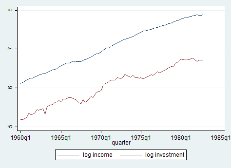
These are Quarterly SA West German macro data from 1960 to 1982 (long before I was born). Remember that, before starting any kind of analysis, you have to tell Stata your dataset is a time series one, using tsset. Taking a look at quarterly investment and real GDP from 1960 to 1982 shows us non-stationary time series having a clear upward trend, even though investments grew less over the period.
Our dataset already contains the first-differenced values of our variables so we can directly proceed to VAR-estimation. We can estimate this model with two fairly simple commands: var and varbasic.
VAR
Let’s start from var, that, without any options it’s just:
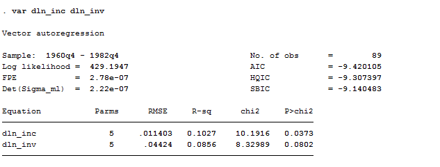
var dln_inc dln_inv
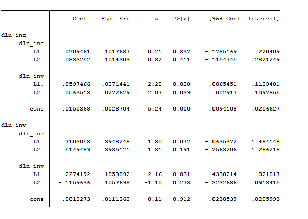
The var command’s output has two parts: a header and the standard Stata output table for the coefficients, standard errors, and confidence intervals. The header contains summary statistics for each equation in the VAR and statistics used in selecting the lag order of the VAR. Given that we did not specify a lag order, Stata automatically perform a VAR with one or two lags. If we want to specify the lags instead, we have to be careful to write the option correctly.
var dln_inc dln_inv, lags(1/2) //tells Stata to include all the lags from the first one to the last one (in our case the second lag)
var dln_inc dln_inv, lags(2) //tells Stata to include just the second lag in the model specification.
Remember that we can use the varsoc command to establish how many lags should be used for a specified model.
VARBASIC
Another useful and more intuitive command to estimate VAR model is varbasic. This command fits a basic vector autoregressive (VAR) model and graphs the impulse-response functions (IRFs) or the forecast-error variance decompositions (FEVDs). The varbasic command simplifies all the procedure. You need to specify the variables in the system and the number of lags to include on the right-hand-side of the model. In our example, only 2 lag are included and the syntax to estimate the VAR is:
varbasic dln_inv dln_inc dln_consump if qtr<=tq(1978q4)
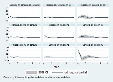
Let’s skip the model part and go directly to impulse response functions, which describe which shock to a system of equations affects those equations over time. In economics we are usually interested in understanding how a sudden and unexpected change in one variable impact another variable over time. Here they are automatically computed by the varbasic command.
Useful Tip: IRFs need to be saved in a file before STATA can access that file and generate graphics. This can be donewith the irf create command like:
irf create datairf, step(9)
Now, I want to generate the impulse response function using the oirf command that yields orthogonal impulse response functions which correspond to selecting a Cholesky decomposition for the contemporaneous effects matrix.
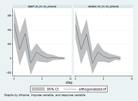
irf graph oirf, impulse(dln_inc) response(dln_consump)
As you can see, the two IRF generated are almost the same! The blue line above represents the impulse response function and the grey band is the 95% confidence interval for the IRF. Notice how at about t= 3 (t is in quarter units) the response declines sharply after having a strong bound and becomes statistically insignificant.The contemporaneous effect of a 10% in differenced income is a little more than 4% for consumption. The effect of an unexpected increase in income would impact consumption immediately and these affects would last about one year.
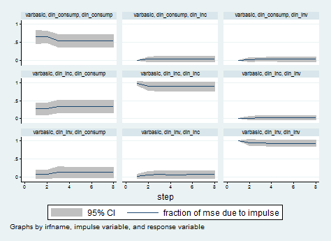
Because we are also interested in looking at the FEVDs, we can use the irf graph command to obtain the graphs like this:
irf graph fevd, lstep(1)
Models with exogenous variables
It’s possible to include exogenous variables in a VAR, simply including the exog() option in the regression. We are already confident with the basic notation so let’s introduce some more option to complicate a bit the stuff!
var dln_inc dln_consump if qtr<=tq(1978q4), dfk exog(dln_inv)
In this case, we tell Stata to consider the first-differenced log transformation of investments as the exogenous variable and we applied the VAR model only to the range period from 1964 to 1978. The dfk option specifies that a small-sample degrees-of-freedom adjustment be used when estimating the error variance–covariance matrix. Don’t panic, I will not deepen this part!
Another interesting option in Stata is to constrain a coefficient of some variables in the equation to zero, so to get rid of insignificant coefficients. Let perform another VAR(2) on a three equation model:
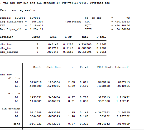
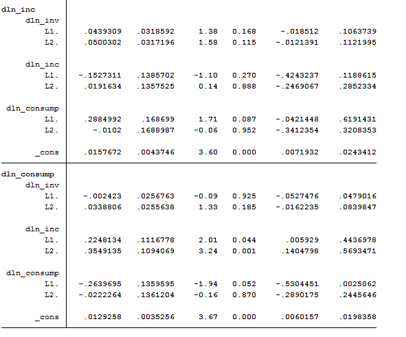
var dln_inv dln_inc dln_consump if qtr<=tq(1978q4), lutstats dfk
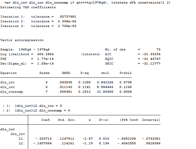
As we can observe, the coefficients in the equation for dln_inv are jointly insignificant, as are the coefficients in the equation for dln_inc; and many individual coefficients are not significantly different from zero. Therefore, we can apply several constraint in order to have a cleaner picture of our data.
constraint 1 [dln_inv]L2.dln_inc = 0
constraint 2 [dln_inc]L2.dln_consump = 0 .
var dln_inv dln_inc dln_consump if qtr<=tq(1978q4), lutstats dfk constraints(1 2)
Post estimation Commands
Predict
The first post-estimation command we must consider is predict, in all its forms:
predict xb, equation(#1)
We are asking Stata to generate the liner prediction for the model. What’s new here, is the equation() option. This is extremely useful when dealing with VAR because allows us to specify for which equation we want to predict residuals, standard error and linear prediction. In this case I asked just for the first equation of my previous three-equation VAR.
VAR Stability
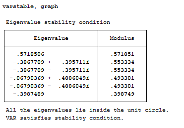
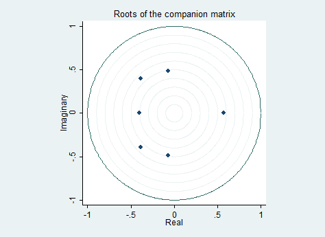
As you know from the theory, to obtain a stable VAR-model we need eigenvalues to be less than one. This can be easily tested with the varstable command, to be run after the estimation. It gives you a table with the eigenvalues for the estimated VAR. All lie inside the unit circle and that’s good for us. If you use the option graph you get graph of the unit circle additional to the output table like this:
varstable, graph
Nice, uh? Extremely useful for presentation also!
Forecast
In order to forecast after a VAR estimation we need to compute the forecast manually through the fcast command:
var dln_inc dln_consump dln_inv if qtr<tq(1979q1) . fcast compute m2_, step(8) . fcast graph m2_dln_inc m2_dln_inv m2_dln_consump, observed><tq(1979q1)
fcast compute f1_, step(8)
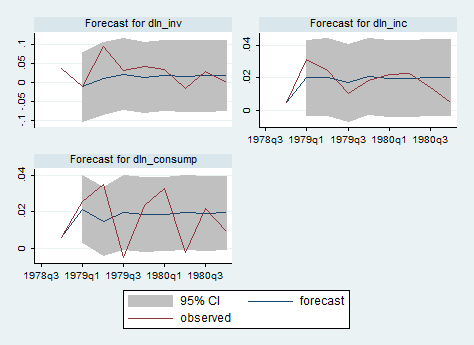
The command fcast compute needs you to specify a suffix (like f1_) to the auxiliary estimations for your regressors because Stata will insert them in your dataset as new variables. The step() option tells Stata to forecast 8 quarters out of the sample. fcast compute creates new variables in the dataset. As you may noticed after having launched the command, fcast compute generates 4 new variables for each dependent variable in your model: forecasted levels, lower bound, upper bound and standard errors. All of these follow the same structure: f1_nameofvariable_UB.
If you want to graph the dynamic forecast you can use the command fcast graph.
fcast graph f1_dln_inv f1_dln_inc f1_dln_consump, observed
The graph shows that the model is better at predicting changes in income and investment than in consumption. The graph also shows how quickly the predictions from the two-lag model settle down to their mean values.
Ok guys for today we are done! If you have any feedback on the topics of these posts or any suggestion on what to cover more, please comment below! Enjoy your sunday!
