As you already know, OLS produces consistent estimates if and only if regression errors are independently and identically distributed. Let’s celebrate the Stata14 release learning something new and extremely important!

Good evening guys!

I am terribly sorry for this prolonged absence but it was a tough month, now I am back in business and today we need to learn what to do when we are aware our errors are not i.i.d.

When this happens, we have two options. First, we can use the robust() option in the OLS model that is a consistent point estimates with a different estimator of the VCE that accounts for non-i.i.d. errors. Alternatively, if we can specify how the errors deviate from i.i.d., we can use a different estimator that produces consistent and more efficient point estimates: the Feasible Generalized Least Square. The tradeoff between these two methods is robustness vs. efficiency. Let’s keep in mind that the i.i.d. assumption fails when:

• The variance of the errors, conditional on the regressors, changes over the observations (not identically distributed). This problem is known as heteroskedasticity and we already saw there how to test for it.
• When the errors are correlated with each other (not independently distributed) but not with the regressors.

We already saw how to deal with heteroskedasticity so I will not spend other words on that unless you need it (If you need it, please leave a comment). However, I want to point out that Stata has implemented an estimator of the VCE that is also robust to the correlation of disturbances within groups and to not identically distributed disturbances, commonly referred to as the cluster-robust VCE estimator that we met in Panel Data analysis there. If in our model the within-cluster correlation are meaningful and we ignore them then our estimates will be inconsistent. Stata’s cluster() option lets you to account for such an error structure. It only requires you to specify a group or cluster membership variable that indicates how the observations are grouped.

The Newey-West estimator

In the presence of both heteroskedasticity and autocorrelation, we can use this consistent estimator (HAC) that has the same form as the robust and cluster-robust estimator. Rather than specifying a cluster variable, it requires that we specify the maximum order of any significant autocorrelation in the disturbance process- known as the maximum lag, L. it is the user’s goal to specify the choice of L. Of course, given that we are talking about autocorrelation, we are already introducing time-series data, which will be the second part taught on my blog, once I finish with the basics. Of course, there will also be a third part. Curios? Stay tuned.

Anyway, this command has the following syntax:

newey y x, lag()

you can use it as an alternative to the regress command and you have to specify the number of lags you want. I am going to use an old dataset that you can find below, named ukrates.dta.

This is a time-series dataset of monthly short-term and long-term interest rates on U.K government securities. The model we want to use expresses the monthly change in the short rates rs (Bank’s of England’s monetary policy instrument) as a function of the prior month’s change in the long-term rate r20 so that this model represents a monetary policy reaction function. I am going to estimate it both with and without HAC standard errors by using regress and newey and then control the estimates. Since we have only 524 observations, we are going to use 5 lags. I will use both the D. (first difference) and L.(lag) operators. That’s what I typed on Stata:

use http://www.stata-press.com/data/imeus/ukrates, clear

regress D.rs LD.r20

estimates store nonHAC

newey D.rs LD.r20, lag(5)

estimates store NeweyWest

estimates table nonHAC NeweyWest, b(%9,4f) se(%5,3f) t(%5,2f)

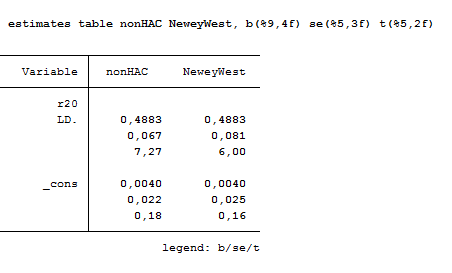
As you can see, the HAC standard error estimate of the slope coefficient from newey is larger than that produced by regress, although the coefficient retains its significance. One issue remain with this estimator. We may want the autocorrelation consistent (AC) estimator without the H. The standard Newey-West procedure as implemented through newey does not allow for this, but the ivreg2 does because it estimates robust, AC and HAC standard errors for regression model. You are kindly asked to review it here.

Feasible Generalized Least Squares

• Heteroskedasticity related to scale

This model allow us to estimate the coefficient of a model where the zero-conditional mean assumption holds, but the errors are not i.i.d. it places more structure on the estimation method to obtain more efficient point estimates and consistent estimators of the VCE.

To use FGLS on a regression equation in which the error process are heteroskedastic we just need to transform the data and run a regression on the transformed equation. The appropriate transformation to induce homoscedastic errors would be to divide each variable in the model by a covariate of the model, obtaining a weighted transformation, thus a Weighted Least Squares regression. Stata implements several kinds of weights and this sort of FGLS involves the analytical aw variety. Let’s use our friend, auto.dta:

regress price mpg weight   // estimate the regression model by OLS and predict the residuals

predict e, residual

generate loge2 = log(e^2) // Use the residuals to estimate a regression model for the error variance

regress loge2 weight foreign

predict zd // and predict the individual error

generate w=exp(zd)

regress price mpg weight [aweight = 1/w] // perform a linear regression using the weights

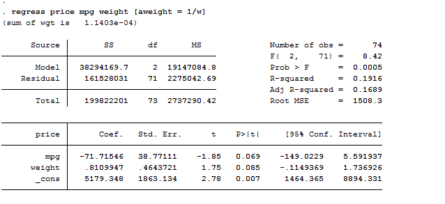
Unlike the first regression, the regression with analytical weights produces the desired measures of goodness of fit and predict will generate predicted values or residuals in the units of the untransformed dependent variable.

• Heteroskedasticity between groups of observations

This happens when we pool data across what may be nonidentically distributed sets of observations. For instance, we might expect with firm data that profits (or revenues) might be much more variable in some industries than others might. Capital-goods makers face a much more cyclical demand for their product than do electric utilities. We can test two groupwise heteroskedasticity with an F test but if we have more than two groups across which we want to test for equality of disturbance variance, things get complicated.

Let’s use another dataset installed in Stata:

use http://www.stata-press.com/data/imeus/NEdata, clear

reg dpipc year

predict double eps, res

robvar eps, by(state)

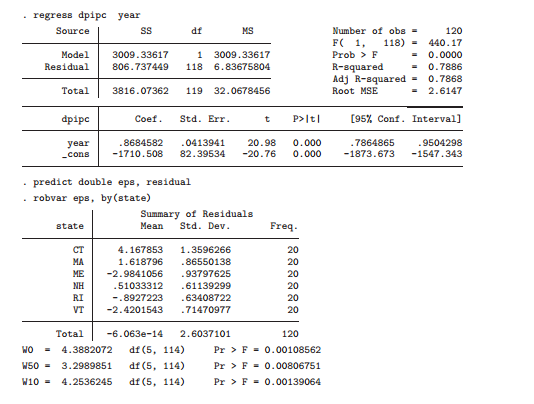
I fitted a linear trend model to state disposable personal income per capita (dpipc) by regressing that on year. The residuals are tested for equality of variances across states with the robvar command. The hypothesis of equality of variances is soundly rejected by all three-test statistics. Then, I estimated the regression with FGLS using the analytical weight series calculated at:

by state, sort: egen ad_eps= ad(eps)

gen double gw_wt = 1/sd_eps^2

reg dpipc year [aw=gw_wt]

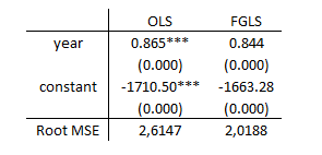
Here we are! Compared with the unweighted estimates’  Root MSE of 2.614, FGLS yields a considerably smaller value of 2.0188.

Enough for today! I will go through the autocorrelation part when I will deal with time-series data! Stay tuned!