Learn Panel Data proficiently on Stata using 5 minutes of your time and you won’t regret it!

Good Morning Guys,

Contrary to what I said up to now, today I am going to provide you a short theoretical explanation of the topic. Why? Because I think, panel data are so important that you cannot allow yourself to do not understand them. Let’s start.

The Theory Behind

Panel data are also known as longitudinal or cross-sectional time-series and are datasets in which the behaviors of entities like States, Companies or Individuals are observed across time. They are extremely useful in that they allow you to control for variables you cannot observe or measure (i.e. difference in business practices across industries) or variables that change over time but not across entities (i.e. national policies) so they control for individual heterogeneity.  Moreover, they allow estimating omitted variable bias when the omitted variables are constant over time within a given state/individual. These data represent the 80% of worldwide data but you must be careful to deal with them due to some drawbacks such as data collection issues (i.e. the sampling design and its replicability), non-response rate (if you have micro data) or cross-country dependency in case of correlation between countries (Macro data). Panel data are usually distinguishable in:

• Balanced Panel: no missing observations
• Unbalanced Panel: some entities are not observed for some time period

Now, let’s make an example. Imagine we can explore if alcohol taxes may be a means to reduce traffic deaths. If we can demonstrate there is a relation, several state policies can be implemented to reduce the number of deaths due to transports. Why might there be more traffic deaths in states that have higher alcohol taxes? Because there are other factors such as density of cars on the road and culture that we are not considering and that determine traffic fatality rate. These omitted variables affect OLS estimates that are no more consistent. That is why we need Panels.

Stata’s Passionate Corner

The first thing we must do when we want to play with Panels in Stata is to use the command xtset; it declares to Stata that we are going to use longitudinal data. Let’s call back the dataset nlswork we already discussed in the OLS post.

webuse nlswork

xtset idcode year, yearly

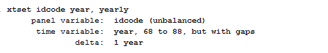
I specified the yearly option to help Stata understanding the time unit is year and not months or days. As we can notice, our panel is unbalanced in the sense that several idcode, which represent interviewed women, have missing observations for some characteristics across the time range.

Useful Tip. If you get the error “string variable not allowed” after using xtset it means that your identifier variable is a string instead it should be a numeric so you can use the command encode, as explained here.

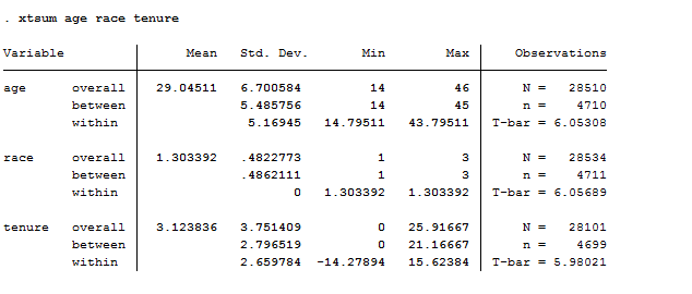
If we want to describe our data, another useful command is xtsum.

xtsum age race tenure

This provides us the mean, the minimum and maximum of the selected variables and the standard deviation. It shows three different estimates. The overall estimate is the total number of individual for the number of years N = n x T. We are dealing with 28500 observations more or less. Between is the estimate that shows between women the number of observations in each characteristics. Within instead shows within each woman the number of observation of the selected characteristics in the time range.

We can also try to understand graphically what we are dealing with. In this case, I recommend you to use the command xtline if you have few observations. I typed:

xtline ln_wage if idcode<10

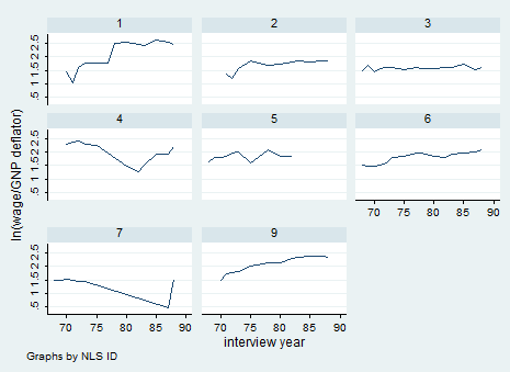
In this case it is not useful because we are using micro data but it may be useful with macro data even with the overlay option so keep it in mind!

Pooled Ordinary Least Square (POLS)

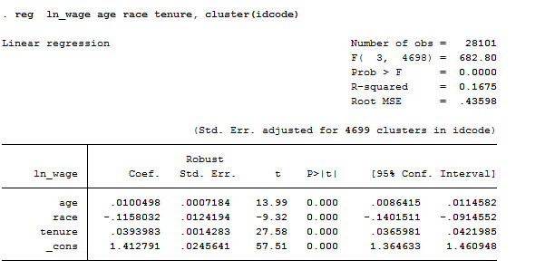
This is nothing more than a simple OLS model once you have declared your data to be Panel. It is the most basic estimator of panel datasets, ignores the panel structure of the data and treats observations as being serially uncorrelated for a given individual with homoscedastic errors across individuals and times. It is useful in microeconometric studies but I do not want to anticipate this topic now! For you it is enough to know:

reg  ln_wage age race tenure, cluster(idcode) // If you suspect there’s correlation across women.

Fixed Effect

I recommend using FE models whenever you want to analyze the impact of variables that vary over time because it explores the relationship between these factors and the outcome variables within entities (i.e. country, person, company). We use them when we believe that something within the individual may bias the predictor or outcome variables and we are not controlling for it. Fixed effect estimation removes the effect of those time-invariant characteristics. The assumption behind is that those time-invariant characteristics are unique to each entity and should not be correlated with other individual characteristics. If the error terms of the estimated regression are correlated, it means that there are individual characteristics that are correlated with characteristics of other individuals so FE is not suitable and you might need to use the Hausman test to check its correctness against a random effect model.

You can use several methods to compute your Fixed Effect model. The first one is using the Least Square Dummy variable regression where dummy variables are created for each entity (except one to avoid multicollinearity) and are included in the model. This technique might be time consuming and it can produce many coefficients that you are not interested in but it is useful to investigate cross-individual correlation! Alternatively, we can add time and entity effect to the model to have a time and entity fixed effect regression model. Finally, we can construct a within regression by demeaning each variable (both regressors and outcome). Hence, within each entity, the demeaned variables all have a mean of zero. You can use this to get rid of all between subject variability.

N.B. if you have time-invariant variables such as gender in your analysis and you apply a demeaned model this demeaned gender variable will have a value of 0 for every individual and, since it is constant, it will drop out of any further analysis.

Before looking at regression command, I am going to give you two way to graphically check if you have heterogeneity across individuals or across years.

The first set of commands allows you to check heterogeneity across individuals so to control for unobserved variables that do not change over time:

bysort idcode: egen race_mean=mean(race)

twoway scatter race idcode if idcode<6, msymbol(circle_hollow) || connected race_mean idcode, msymbol(diamond) || , xlabel( 1 “A” 2 “B” 3 “C” 4 “D” 5 “E”)

The second set of commands allows you to control for unobserved variables that do not change over time.

bysort year: egen race_mean1=mean(race)

twoway scatter race year if idcode<6, msymbol(circle_hollow) || connected race_mean1 year, msymbol(diamond) || , xlabel(68(1)88)

Here we are! Let’s start with regressions.

Least Square Dummy Variables (LSDV)

We first have to create a dummy for each observations. Given that this dataset it is unfeasible as it is now (N=4899) I am going to drop most of the observations through:

drop if idcode>10

Then I generate the dummy variables, one for each woman:

tabulate idcode, gen(id)  or

xi i.idcode

You can use both these commands to create dummy variables but the second one does not save the new variables permanently, as the first does. On the contrary, the strength of the second is that it directly creates N-1 dummies to avoid multicollinearity whereas tabulate computes all of them. Finally yet importantly, you can use the xi command as a prefix too:

xi: reg ln_wage age race tenure i.idcode // Direct regression with dummies without inserting them in the dataset

then:

reg ln_wage age race tenure id2-id9

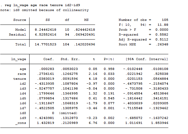
This regression is useful if you want to know if the difference in women effects is statistically significant. We include the intercept and the dummies (except one) however, one of the dummies is dropped due to perfect collinearity of the constant and all the other dummies are represented as the difference between their original value and the constant. Otherwise, we can calculate the fixed effects model including dummy variables for each woman instead of a common intercept. The only change is the substitution of a common intercept for 8 dummies, each of them representing a cross-sectional unit. It provides a good way to understand fixed effects because the effect of age, for example, might be mediated by the differences across women. By adding the dummy for each woman, we are estimating the pure effect of age.

Within Regression

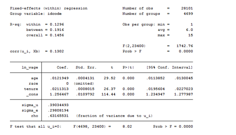
The regression command for panel data is xtreg. You can either type:

xtreg ln_wage age race tenure, fe  cluster(idcode)// without the fe option by default is random effect

or using another command that is areg, which syntax is:

areg ln_wage age race tenure, absorb(idcode)

As we can see from the table below, the xtreg model suffers of collinearity. The intercept is an average of individual intercepts.

When using areg you always have to specify which variable you want to absorb. The common practice is to generate the dummies for each observation and absorb them. Even though they are not displayed, the overall F-test of the model report their presence.  Areg has three different syntax you can use. I report them ordered:

• areg ln_wage age race tenure, absorb(idcode) r cluster(idcode)
• areg ln_wage age race tenure, absorb(idcode) r
• areg ln_wage age race tenure, absorb(idcode)

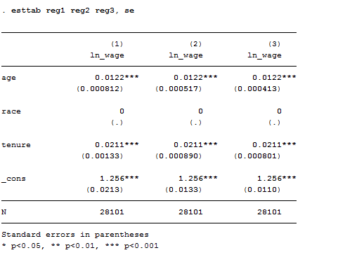
As we can see from the table constructed using estout the third model is the one that better fit out data. The underlined hypothesis is that we are not facing serial correlation neither heteroskedasticity.

Between-Groups Estimator

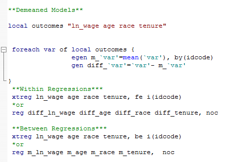
To perform a between model you can use the be option after xtreg or construct a demeaned model in the do-file that you might also use it for within estimation.

Random Effects

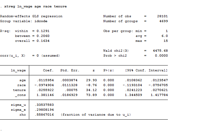
In this case, the variation across entities is assumed to be random and uncorrelated with predictors or the outcome variable. . Its advantage is that we can include time invariant variables like gender because it assumes that the entity’s error term is not correlated with the predictors. You can estimate random effect directly typing xtreg or adding the re option.

xtreg ln_wage age race tenure

Hausman Test

quietly xtreg ln_wage age race tenure, re

eststo re_reg

quietly xtreg ln_wage age race tenure, fe

eststo fe_reg

hausman fe_reg re_reg

The Hausman test allows you to decide between fixed or random effects. Its null hypothesis is that the preferred model is random effects and it tests whether the unique errors are correlated with the regressors. If the model that fit better the data is a random effect than the null hypothesis is that the errors are uncorrelated. If the Chi-statistic is negative then the test is not conclusive.

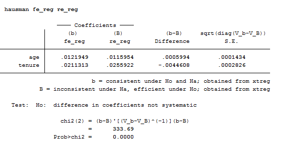
In our case, we should prefer and use a fixed effect model.

Testing for Time-Fixed Effects

If we are not sure that we need to control for time fixed effects when running a Fixed effect model, we can use the command testparm that performs a joint test of significance. You can check if the dummies for all years are equal to zero.

xtreg ln_wage age race tenure i.year, fe

testparm i.year

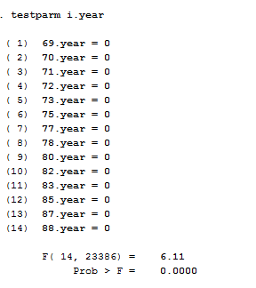
Considering that the Prob>F is smaller than alpha (0.05) we reject the null hypothesis that the coefficients for all years are jointly equal to zero confirming that time fixed-effects are needed in our case.

Testing for Random Effects

The Breusch-Pagan Lagrange Multiplier test is what we need to decide between a random effects regression and a simple OLS regression. Its null hypothesis is that variances across entities is zero. Thus, there are not panel effect because there is no significant difference across units. The command in Stata is xttest0.

xtreg ln_wage age race tenure, re

xttest0

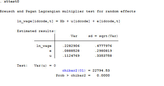
Here we reject the null and conclude that random effects is the appropriate model because there is evidence of significant differences across women. As a result, OLS is biased.

It’s All for Today! Stay tuned for more posts.