Have you ever wondered how to make regressions and test them using Stata? If the answer is Yes, read below…

Good morning Guys!

Today we are ready to start with the grass-roots econometric tool: Ordinary Least Square (OLS) Regression! We will revise several commands that I already described in previous posts so, in case you missed them, you have the opportunity to review them again.  I am sorry but I am not going to give you a theoretical explanation of what we are doing so, if you are not familiar with the argument yet, I suggest you to check The Econometrics’ Bible: Wooldridge. I am only going to discuss some modeling strategy.

A Piece of Theory: Modeling Strategies

One of the assumptions of the OLS model is linearity of variables. However, if we abandon this hypothesis, we can study several useful models whose coefficients have different interpretations.

Log-log model

In this model, both the dependent and independent variables are logarithmic.

In our example, I have log transformed a hypothetical writing and math scores test. In this model, the beta coefficient may be interpreted as elasticity of lwrite respect to lmath. Indeed, beta is the percent variation of lwrite associated with a 1% variation of lmath.

Log-lin model

Very often, a linear relationship is hypothesized between a log transformed outcome variable and a group of predictor linear variables likes:

Since this is just an ordinary least squares regression, we can easily interpret a regression coefficient, say β1,  as the expected change in log of write with respect to a one-unit increase in math holding all other variables at any fixed value.

Lin-log model

This model is the opposite of the previous one. The regressor is log transformed while the dependent variable is linear. Beta can be interpreted as the unitary variation of write score respect to the relative variation of the math score.

Quadratic Model

In this model, one of the independent variables is included in its square as well as linear terms.

The marginal effect of age on wage depends now on the values that age takes. This model is usually described with graphs of trajectory.

Model with interactions

If we want to compute an interaction term between two independent variables to explore if there is a relation we can write:

In this model, the β1 coefficient can be interpreted as the marginal effect age has on wage if race=0. The marginal effect depends on the other regressor. (i.e. Marriage premium).

Choose the Correct Functional Form

My personal opinion is that we should choose the model based upon examining the scatterplots of the dependent variable and each independent variable. If the scatterplot exhibits a non-linear relationship, then we should not use the lin-lin model. Given that sometimes we have huge amounts of data, this procedure becomes unfeasible. We can try to follow the literature on the topic and use the common sense or decide to compare the R-Squared of each form as long as the dependent variables are the same. You should choose the model with the higher coefficient of determination in this case. An incorrect functional form can lead to biased coefficients, thus it is extremely important to choose the right one.

Make your Regressions

In order to investigate some interesting relations we must abandon our auto.dta dataset and use a subsample of Young Women in 1968 from the National Longitudinal Survey(nlswork) available by typing:

use http://www.stata-press.com/data/r12/nlswork.dta

If you want to describe data, type describe and you will see that this is a panel data of women of 14-26 years providing information regarding their race, marital status, educational attainment and employment. I am not going to discuss panel data now but it is good if we start to know the database that I will use in the next posts to introduce panel data.

Regress

With the –regress- command, Stata performs an OLS regression where the first variable listed is the dependent one and those that follows are regressors or independent variables.

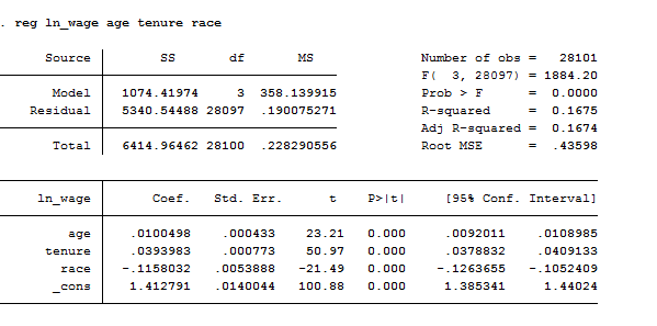
Let’s start introducing a basic regression of the logarithm of the wage(ln_wage) on age(age), job tenure(tenure) and race(race). Please notice that we have a logarithmic measure of wage, this means we are going to study elasticities or semi-elasticities estimates. If we type:

reg ln_wage age tenure race

This is the output produced by Stata:

If we want to know which objects from this regression Stata automatically saves, we need to type:

ereturn list     // It shows saved estimation objects

If, on the opposite, we want to select which estimates need to be shown and then saved, we can type:

matrix list e(b)       // shows the vector of coefficients

matrix list e(V)       // shows the var-cov matrix of coeff

matrix V=e(V)    // saves e(V) with the name “V”

Why we might need to save these estimates? Well, maybe we want to type directly just the standard error and t-statistic of one of the independent variables. How? Easy:

scalar SE_age=V[1,1]^.5

scalar t_age=b[1,1]/SE_age

scalar list SE_age t_age

In addition to getting the regression table, it can be useful to see a scatterplot of the predicted and outcome variables with the regression line plotted.  After you run a regression, you can create a variable that contains the predicted values using the predict command.  You can get these values at any point after you run a regress command, but remember that once you run a new regression, the predicted values will be based on the most recent regression. To create predicted values you just type predict and the name of a new variable Stata will give you the fitted values. For example:

predict fitted

We can also obtain residuals by using the predict command followed by a variable name, in this case e, with the residual option:

predict e, res

If we want to understand with a graph what we have created, we can either type:

scatter ln_wage age || line fitted age    or

rvfplot, name(rvf) border yline(0)  // Plot of residual vs. fitted

lvr2plot, name (lvr) // residuals vs. predictor

graph combine scatter rvf lvr 

Did you miss my post on graphs and you are lost? Check it out now here.

The regress command by default includes an intercept term in the model that can be dropped by –nocon– option. Other options such as beta or level() influence how estimates are displayed; beta particularly gives the standardized regression coefficient.

Heteroskedasticity

If we want to examine the covariance matrix of the estimators to see if homoscedasticity is respected, we can add the vce() option.

You can observe the presence of heteroskedasticity by either graphs or tests. The command to ask Stata to perform a White test is:

imtest, white

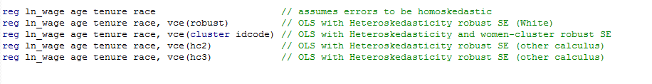
The null hypothesis of this test is homoscedasticity. If we find heteroskedasticity, then we can adjust the standard errors by making them robust standard errors. Another test to control for heteroskedasticity is:

estat hettest

I suggest you to check this out because it has several interesting options. We can also correct for it by utilizing the Weighted Least Squares (WLS) estimation procedure that is BLUE if the other classical assumptions hold (see the theory to understand what BLUE means). To compute the Weighted Least Squares (WLS) you have to add as an option in brackets the variable by which you want to weight the regression, like:

reg ln_wage age race tenure [aw=race]

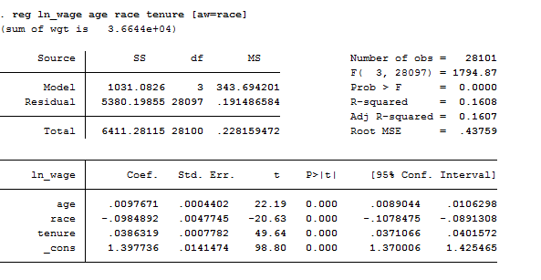
Once we fit a weighted regression, we can obtain the appropriately weighted variance–covariance matrix of the estimators using estat vce and perform appropriately weighted hypothesis tests using test. Regress supports also frequency weights ([fweight=age]).

 Tests

Test of Hypotheses

Finally, after running a regression, we can perform different tests to test hypotheses about the coefficients like:

test age                    // T test

test age=collgrad   //F test

test age tenure collgrad // F-test or Chow test

 Test on the Specification

Endogeneity

The Regression Equation Specification Error Test, Ramsey Test, allows you to check if your model suffers from omitted variable bias. You can easily understand it if your coefficients are unusually large (or small) or have an incorrect sign not conform to economic intuition. In this case, the command you are looking for is:

estat  ovtest

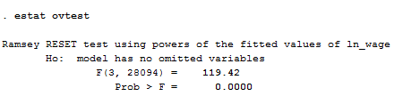
As we can see from the result, given that P-Value<alpha, we reject the null hypothesis that the model has no omitted variables. Thus, we need to try a different specification because rejection of the null hypothesis implies that there are possible missing variables thus the model suffers from endogeneity, causing biased coefficient estimates.

Autocorrelation

Serial correlation is defined as correlation between the observations of residuals and may be caused by a missing variable, an incorrect functional form or when you deal with time series data. In order to test for autocorrelation we can use the Breusch-Godfrey Test. Its command is:

estat bgodfrey

The null hypothesis is that there is no serial correlation. If we find it we can correct for it by using the command –prais– rather than –regress-. Another way to test for first-order autocorrelation is to implement the Durbin_Watson test after the regression, using the command:

estat dwatson

 Normality

If you want to test if the residuals of your regression have a normal distribution the first thing you need to do is to use the –predict- command to save them with a proper name and then you can type:

sktest res

This command can be used also to investigate if your variables are skewed before regress them. If we get back a second to the auto database, this is what appears when you compute sktest:

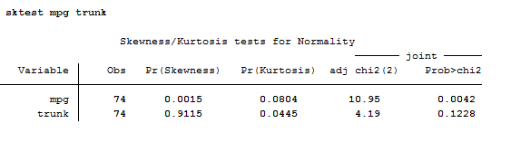
As you can observe, sktest presents a test for normality based on skewness and another based on kurtosis and then combines the two tests into an overall test statistic.  Pay attention because this command requires a minimum of 8 observations to make its calculations.

Multicollinearity

If your regression output displays low t-statistics and insignificant coefficients it might be that, you have selected as independent variable to explain your output, variables that are perfectly correlated among them.

The first thing I suggest you to do is to examine the correlation matrix between the independent variables using the –correlate-command.

corr age tenure race

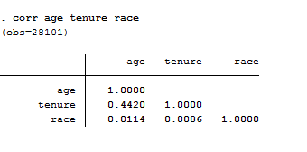
Even thought I was sure that our regressors were uncorrelated I checked them out. As a rule of thumb, a correlation of 0.8 or higher is indicative of perfect multicollinearity. If you do not specify a list of variable for the command, the matrix will be automatically displayed for all variables in the dataset. Correlate supports the covariance option to estimate covariance matrix and it supports analytic weights. Another useful command you must check is pwcorr that performs pairwise correlation.

pwcorr age tenure race

The correlations in the table below are interpreted in the same way as those above.

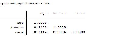
The only difference is the way the missing values are handled.  To compute a correlation you just need two variables, so if you ask for a matrix of correlations you could just do so by looking at each pair of variables separately and include all observations that contain valid values for that pair. Alternatively, you could say that the entire list of variables defines your sample, in that case would first remove all observations that contain a missing value on any of the variables in the list of variables. -pwcorr- does the former and -corr- does the latter. When you do pairwise deletion, as we do in this example, a pair of data points are deleted from the calculation of the correlation only if one (or both) of the data points in that pair is missing.  There are really no rules to define when use pairwise or listwise deletion.  It depends on your purpose and whether it is important for exactly the same cases to be used in all of the correlations.  If you have lots of missing data, some correlations could be based on many cases that are not included in other correlations.  On the other hand, if you use a listwise deletion, you may not have many cases left to be used in the calculation.

If you don’t remember how to control if your variables present missing values you are kindly advised to read here.

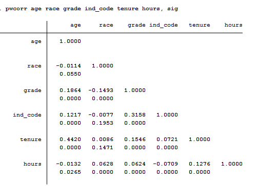
In the example above, variables age and tenure are the only variable with missing values. Pwcorr supports also the sig option that allows Stata to display and add significance level to each entry like that:

Too much information to digest? I hope not! Stay tuned for the next post on Logit and Probit Models.