Sometimes your variable are not good enough to predict an outcome and you need to find a replacement to instrument them. Make your models work on Stata!

Good morning guys!

Today we are going to study a group of variables that I personally dislike: endogenous one. When you have an endogenous regressor, your OLS estimates become inconsistent and it may happen thanks to measurement error or omitted variable biases. That is why we need to find another variable, called an instrument, that is exogenous and it is correlated with the outcome variable only through its effect on the endogenous regressor. For a review of the theory, please check Green or Wooldridge’s books. Are you ready to play with them?

We will need to use a special database named card.dta that you can download from:

http://www.stata.com/texts/eacsap/

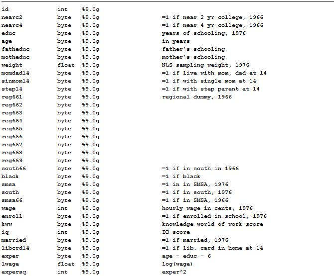
This dataset contains information on a sample of 3010 working men aged between 24 and 34 who were part of the 1976 wave of the US National Longitudinal Survey of Young Men and it is usually studied to replicate the estimates of the earnings equations. It includes a measure of the log of hourly wages in 1976 (lwage), a measure of years of education (educ), years of labour market experience (exper), the square of years of labor market experience (expersq) and other useful variables we can look at through the describe command:

We want to investigate returns to schooling that means how much your earnings can increase if you spend more years of your life to study and form yourself at school. If we want to study the sign of this relation, the perfect starting point is a scatter plot.

graph twoway scatter lwage educ || lfit lwage educ

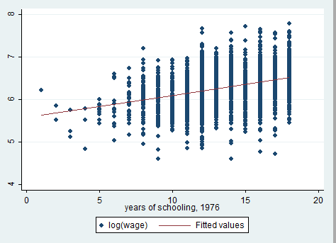
The relationship is positive! The question is:  is education an exogenous regressor? The answer is likely to be NO, because of other confounding variables such as ability that affect both education and earnings. We will use proximity to college (nearc) as an instrumental variable for years of education (educ), replicating Card’s study (1995). The idea is that, being all else equal, individuals are less likely to choose college education if they live far away from a suitable college. Assuming that the presence of a nearby college is uncorrelated with ability (controlling for family background factors), college proximity is a potential instrumental variable for schooling. Does it seem reasonable to you?

Let’s first investigate the OLS model. We already said that it should be inconsistent but let’s look at the data:

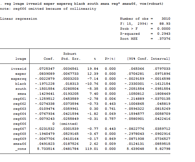
reg lwage educ exper expersq black south smsa reg* smsa66, vce(robust)

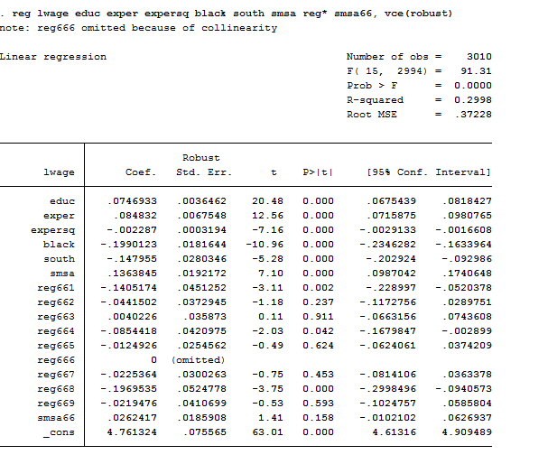
As we can observe, one of the regional dummies was dropped due to multicollinearity because we inserted the intercept. If you missed this point, you can review the theory here. The coefficient of education is positive and significant meaning that one-year more of schooling implies an increase of 7.4% in return to schooling (or wage). Remember that this is a log-lin model that we studied here, so its coefficients should be interpreted with caution.

Two Stage Least Squares (2SLS)

First Stage

This method allows you to introduce instrumental variables in your regression model and is named like that because it is a two-step procedure. In the first step, we are going to regress the endogenous variable on all its possible instruments. Here we want to check that the instruments have explanatory power so that they are both valid and informative:

reg educ nearc2 nearc4

testparm nearc2 nearc4

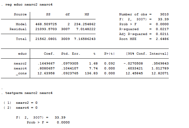
As we can see, both nearc2 and nearc4 are predictive of education, individuals who lived near to a college were significantly more likely to choose additional education. How can we state if they are good instruments? The problem with instrumental variables is that we cannot choose weak instruments for our explanatory variables because it could lead to worse estimates than OLS, already biased. Weak identification arises when the excluded instruments are correlated with endogenous regressors, but only weakly. Estimators can perform poorly when instruments are weak and different estimators are more robust to weak instruments than others are. The rule of thumb is that, if F>10 (it is 33.4 in our case) then the instrument is strong. Testparm, which we introduced with panels, is a post estimation test that works like an F-test on joint significance of coefficients. From the first-stage regression, we can estimate residuals:

predict ivresid, res

est store ivreg

Second Stage

Now we can use OLS to estimate the second stage regression including the estimated residual of the first-stage to the education variable like this:

reg lwage ivresid exper expersq black south smsa reg* smsa66, vce(robust)

We should obtain the same estimated coefficients with two other packages: ivregress and ivreg2.

Ivregress

This is the Stata’s basic command to compute IV estimates that has substituted the previous ivreg command. Ivregress can fit a regression via 2SLS but also via GMM (generalized method of moments, we will address this topic in another post), so if we want to use 2SLS we have to specify it. It can directly shows the estimates of both the second and the first stage by imposing the first option. Ivregress works with brackets where you can type a list of variable names both before and after the = sign. The variables putted in brackets before the = sign are the explanatory variables that you believe are endogenous; the variables putted in brackets after the = sign are the instruments.

Useful Tip: You can have more than one instrument for a single endogenous variable as in this example. In this case, the strongest instrument you can obtain is the linear combination of the instruments.

Useful Tip 2: if we have more than one endogenous variable there’s a condition known as rank condition that requires at least as many exogenous variable (instruments) as the endogenous variables are.

In our case the syntax of the command is:

ivregress 2sls lwage exper expersq black south smsa reg* smsa66 (educ = nearc2 nearc4)

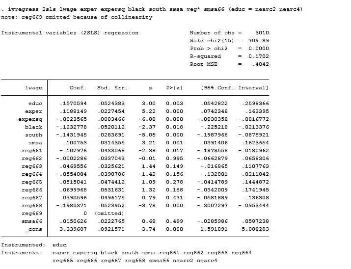
As we can observe, now that we have instrumented education, the estimates of the return to schooling exceed the corresponding OLS estimates by almost 50 percent (15,7% vs 7,4%). If we assume a priori that OLS methods lead to upward-biased estimates of the true causal effect of schooling then, larger IV estimates are puzzling. In this case, the estimates can be interpreted by saying that individuals who lived near to a college were significantly more likely to choose additional education and have better salaries.

Ivreg2

You must install this package on Stata if you want to use it. I recommend you to check it out because it provides a more powerful alternative to Ivregress. Indeed, it also provides tests of over-identifying restrictions and implements various test for under-identification or for weak instruments. If you specify the ffirst option it also computes test for the first stage. For example:

ivreg2 lwage (educ = nearc2 nearc4) exper expersq, ffirst

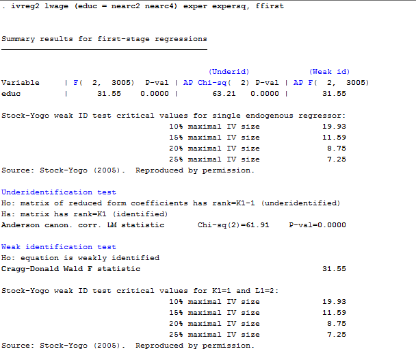
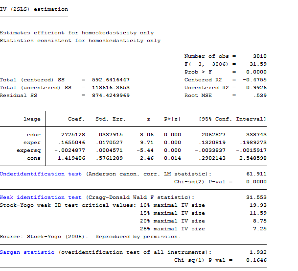
From the output we can say that our model do not suffer from under identification nor of weak instruments’ choice.

Useful Tip: testing of over-identifying assumptions is less important in longitudinal applications because realizations of time varying explanatory variables in different time periods are potential instruments.

Useful Tip 2: in the presence of conditional heteroskedasticity, the Sargan test is not robust and should not be used. If this is the case, you can use the test proposed by Hansen that is a heteroskedasticity-robust test of over-identifying restrictions.

How can we test if we are facing endogeneity?

Hausman Test

This test that we already mentioned in panels, evaluates the consistency of an estimator when compared to an alternative, less efficient, estimator that is already known to be consistent. It helps to evaluate if the IV model correspond to the data better than an OLS one.  Under the null hypothesis both the OLS and IV estimators are consistent but only the OLS estimator is efficient (has the smallest asymptotic variance). Under the alternative hypothesis, the IV estimator is consistent and efficient. If the null is rejected, then either (i) the instruments are endogenous and the covariates are endogenous or (ii) the instruments are exogenous and the covariates are exogenous or (iii) the instruments are endogenous and the covariates are exogenous.

This test can also be used to check the validity of extra instruments by comparing IV estimates using a full set of instruments Z to IV estimates that use a proper subset of Z. in this last case we must be certain of the validity of the subset of Z. Moreover, that subset must contain enough instruments to identify the parameters of the equation. The syntax is:

reg educ nearc2 nearc4

est store ivreg

reg lwage educ exper expersq age married smsa

Hausman ivreg ., constant sigmamore  

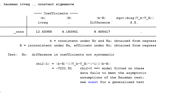
I specified the constant option to tell Stata to include the constant of the two equations and the sigmamore option that bases both covariance matrices on disturbance variance estimate from efficient estimator. It is not strange that the test failed producing a negative chi-squared statistics. This may happen because the assumption that one of the estimators is efficient is a demanding one. If the observations are clustered or pre-weighted, this will fail for sure and the test will be undefined. Stata supports a generalized Hausman test, suet that overcomes both of these problems. There is another way to obtain the Hausman test. If you use ivreg2 you just need to specify the regressors to be tested in the orthog() option.

Last question: How can we find a good instrument? Well, if you are able to find a strong instrument that is also unknown to the previous literature on your topic you can directly apply for a PhD because your research will be published for sure. Finding instruments is a tough job and several of them are strange or unbelievable. Consider this one:

Have you ever imagined that settler mortality in French and English colonies could have helped predicting the current performance of institutions in those territories? If not only you can picture this but it also seems straightforward to you then, my friend, you are likely to make friendship with this nice guy:

Daron Acemoglu