Moving average and exponential smoothing forecasts are closely related extrapolative techniques that uses averages of the most recent data to calculate forecasts. Today let’s discover how to apply exponential smoothing on univariate time series.

Good afternoon guys,

I hope your Sunday afternoon isn’t rainy as mine is. But that’s still good, because it can be the right time to write something valuable.

So, today’s focus is on exponential smoothing techniques that is basically the alternative to ARIMA model. As said so far time series models are used to understand the underlying structures and forces in which an observed dataset has its root. They also allow us to fit a model and then proceed to its monitoring and forecasting, thus guaranteeing a broad vision on what’s going on around.

What we probably ignore is that there exist four models of exponential smoothing: a simple one used to model series with no trend neither seasonal variation; the Holt one, which posits that series have a linear trend and no seasonal variation; the Winters one (it’s plenty of famous people here!) where it’s supposed that the series has both a linear trend and a multiplicative seasonal variation and finally the custom one that is basically the one in which you can specify everything from trend to seasonality.

In order to deeply explore their features, I chose a unique firm’s sales data of thirteen variables to forecast its monthly sales from 1988 to 1998. We are going to analyze the men’s clothing line so, my fellow female friends, let’s get thrilled! The first thing to do is to import my .csv file into Stata, using the proper command:

import delimited C:\Users\Michela\Desktop\seasfac.csv

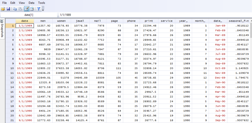
As you can see, the dataset is quite simple. We have number of pages ‘catalogs, catalogs mailed, number of phone lines opened for orders, amount spent on print advertising and seasonal factors for sales of men’s clothing. There’s a problem though, our data variable is a string one. So, the first thing to do is to create our numerical data variable, with the command studied before (you can find it here):

gen mydate=ym(year_,month_)

format mydate %tm

tsset mydate, monthly

Why am I specifying this? Because I want to understand with a graph how our sales are going 😉

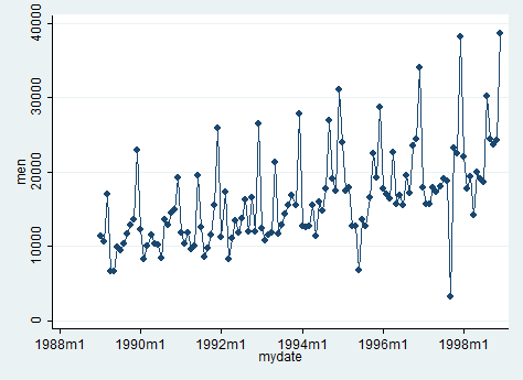
scatter men mydate, c(l) sort

As we can observe, through the peaks that might reflect seasonality, sales are increasing in the range period selected.

PRELIMINARIES

Now that we observed this, we have to analyze if there is a clear trend and in which direction it goes if any. In order to do so we can use the dickey-fuller test that we already explained here.

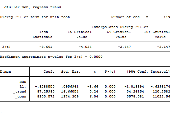
dfuller men, regress trend

WOW! It seems we had the right intuition. Here we are, our series display a positive trend and a unit root (of course, it’s non-stationary) so we have to first-differentiate it. Let’s also try to detect seasonality with a couple of passages:

reg d.men l.men

predict res, r

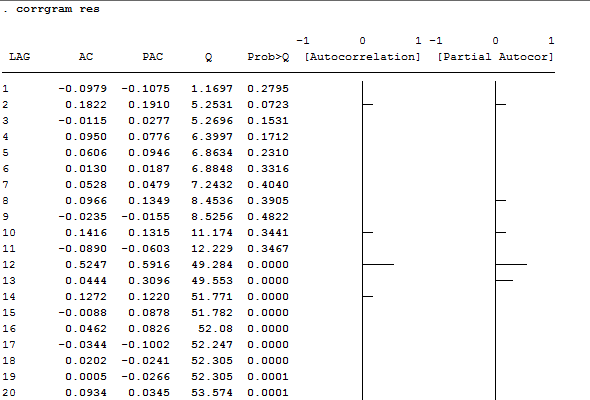
corrgram res

Both PAC and AC plot highlight the annual seasonality’s structure of the time series. Another look at the Q statistic reveal us the need to test for white noise, using the wntestq command.

wntestq res

The test is significant at a 0.05 p-value so residuals are correlated. Believe me even though I am skipping the display of this one.

MODELS

These checks were noisy but necessary to understand which of the 4 models described so far can be adopted in this situation. As we said, we need to construct a model who can deal with both trend’s presence and seasonality thus we have to go for the Winters one. Just to be comprehensive I will show you also the commands for the other variants.

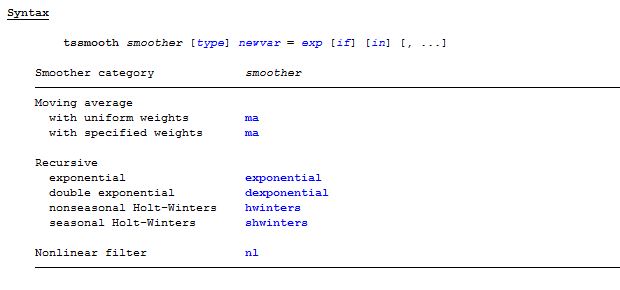
In case you want to model a single exponential smoothing, all you need to do is to run the tssmooth command, whose basic syntax is:

So, we implement the simple model as follows:

tssmooth exponential men1=men

A simple exponential smoothing model adjust forecasts according to the sign of the forecast error; the smoothing parameter is known as alpha and it’s a number between 0 and 1. The smaller the alpha the less the forecast will change so the more dramatic the changes in the series are, the higher the alpha should be.  The command is straightforward but we already know this isn’t the model we need to finish our job. What we need is tssmooth hwinters, which is used in smoothing or forecasting a series that can be modeled as a linear trend in which the intercept and the coefficient on time vary over time. With Holt-Winters non-seasonal smoothing we can decide to either specify our parameters or let them being established by the recursive path:

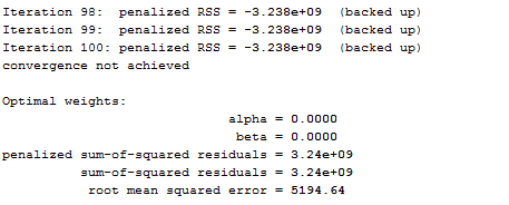
tssmooth hwinters men2=men, from(.1 .1) iterate(100)

Here, I am telling Stata to create a new variable from the original one (to compare different model without replacing existent data). The from() option allows me to use the values I decided 0.1 to be the starting values for the parameters to be estimated whereas the iterate option it’s asking to implement a recursive path 100 times.

Useful Tip: Remember that you must tsset your data before using the tssmooth command.

Of course, this model is incorrect to fit our data because we already saw that we need to account for seasonality. Therefore, we are going to use the Holt-Winters seasonal model, which command is:

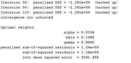
tssmooth shwinters men3=men, sn0_0(seasonal_factors_men) forecast(12) from(.1 .1 .1) iterate(100)

Again we have established parameters, iterations but now we asked for twelve steps ahead forecasts and to use initial seasonal values in the seasonal_factors_men variable included in the data. sn0_0 specifies the initial seasonal values to use of the variable, which must contain a complete years’ worth of seasonal values, beginning with the first observation in the estimation sample.

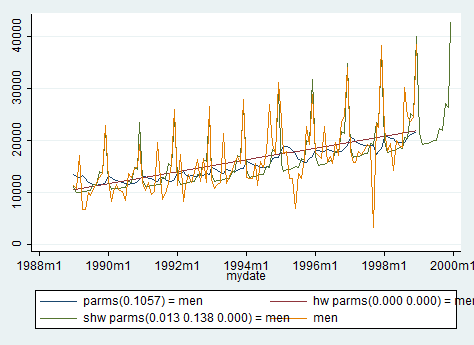
Everything we can do now is to compare graphically the features of the three models estimated before, using the line command.

line men1 men2 men3 men mydate

Men’s clothing sales are forecasted to increase further in the following months. Brand managers can be proud of this and breathe normally for another semester!

Ok guys. Time to rest now! I hope to receive your feedback and see you soon on the next topic!!