Anytime you want to check if you are approaching the problem, just display graphs and tables on Stata.

Good morning Guys!

I hope you are surviving this new week. As I mentioned in the previous post, I am going to follow up on the discussion regarding how to professionally present your data.  Today we are going to play a bit with  tables  and review several helpful commands to produce publication-style tables.  Let’s start from the usual and friendly auto.dta!

There are several ways to access information stored after having run a command. As I already discussed before, the first useful command to store data saved in Stata is outsheet. Given that I already presented it, I will not spend a word on this command and just make an example.

keep make price mpg rep78 foreign // I keep only these 5 variables

keep in 1/10 // I retain just the first tenth observations

outsheet using exampletable.xls

type exampletable.xls

The proof of the pudding!

Packages that save your life

Stata has several packages that you can install to create professional tables of descriptive statistics or regression analysis. I am going to present you tabout, estout and outreg. With these three packages, you can compute interesting stuff and cover everything you need to create!

Useful Tip: When you want to install a package that is not already included in Stata you can either type findit package or write:

ssc install tabout

An opened window will appear on the screen where you must click the blue text (click here to install) to proceed with the installation of the packages you need.

Tabout

Ian Watson developed this package and saved my life during the first years of university. Its syntax is:

tabout foreign rep78 using table11.xls, c(mean mpg mean weight mean length median price median headroom) f(1c 1c 1c 2cm 1c) clab(MPG Weight_(lbs) Length_(in) Price Headroom_(in)) sum npos(tufte)

This is more or less comprehensive of all the disposable options. I am asking Stata to display in an .xls table (you can also specify .out or .csv file if you need it) where the columns represent the mean and the median of several variables divided for type of cars and with five frequencies of repairs. I assigned the labels and told Stata to construct a summary table (sum) with different columns headings (clab). In your directory now you can find an excel file named “Table1.xls”, as a result of this command. To see and learn other useful options, I recommend you to check the help tabout command window. I suggest you to use this command if you want to produce descriptive and summary tables.

Outreg2

This package allows you to save the output of regressions, I will also cite it in the next post on regressions so that you can have a comprehensive and clean picture of what we are doing. For now, let’s say that it can also be used to obtain tables of descriptive statistics and  it produces tables in Word, Excel, LaTeX, and text format. outreg2 also comes with –shellout– command that directly opens the produced tables in Word, Excel, or LaTeX (or TeX-associated editors) for the users of Window XP. This is very fast and a useful tool during research. A blue hypertext is also produced, which you can click to activate. Finally, outreg2 comes with –seeout– command that immediately displays the produced table in the browser view within Stata.
This package is a research tool to be used during research, not after. Making regression tables is not something you would perform only at the end of research. Without undue effort on your part, outreg2 gives you the immediate access to a formatted table that let you compare across regressions on the computer screen.

Its usual syntax is:

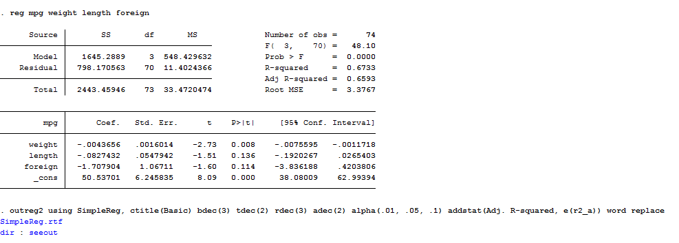
reg mpg weight length foreign

outreg2 using SimpleReg, ctitle(Basic) bdec(3) tdec(2) rdec(3) adec(2) alpha(.01, .05, .1) addstat(Adj. R-squared, e(r2_a)) word replace

What does it mean? You have to decide the name of the file you want to create (i.e. SimpleReg), assign a title to the columns of this file with the ctitle option, and specify the number of decimals to be shown in the coefficients, t-statistics, errors and the significance levels alpha. If you want more statistics than the R-squared, you can use the addstat option and specify them (i.e. adds(F-test, r(F), Prob> F, r(p)’), you can also want the variables to be named after their labels rather than names. In this case you must specify the label option.  The final part is the key one. Here I chose a word format thus, I wrote word but I could have also specified it directly like myreg.doc. The replace option is added because I wanted to replace the file with the same name. Another important option is append. Append should be used when you want to launch outreg2 and store several regression outputs in the same matrix so you tell the package to add these regressions in the same file. Finally, another option I did not specify here is sideway that requests the standard errors to be placed to the right of the coefficients.

As you can see from this do-file, I have created two different files of output, one in word, which contains three regressions, and the other one in excel with a single regression. Please do not panic about all the regression options you do not know. It’s the next argument we will explore, just have patience.  I suggest you to use this command if you need to store and export regressions in another format.

Useful Tip: If you open the output file outreg2 creates you cannot launch the command again with the option append or replace. If you want to add a model with append please make sure that you closed the file myreg.doc Before! Otherwise Stata will give you an error displayed in red.

Estout

This is the final command I am going to introduce. I left it at the end because the estout package has several features that can be combined to produce different kind of tables. Once you installed estout, you can observe you may use these commands: estout, estadd, eststo, esttab, estpost. Let’s explore them all with several examples.

Tables of Contents

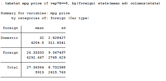
Let’s say we want to check the difference in mean between two variables depending on a condition. The command is tabstat:

tabstat mpg price if rep78==5, by(foreign) stats(mean sd) columns(stats)

As we can see, we have created something that is easy-to-read but of ugly appearance. Moreover I did not tested yet the difference in means. I can use estpost to compute this test. The estpost command takes the results of several common summary statistics commands and converts them to formats that will be used by esttab. Estpost works with various commands like summarize, tabstat or tabulate. In this case I want it to post two-group mean-comparison test, thus its syntax becomes:

estpost ttest mpg price if rep78==5, by(foreign)

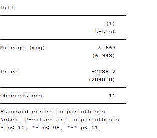
You might say this is ugly as well. You are right but now we have all we need to produce a table of differences in means-We can use esttab to show in a professional way the estimates stored or obtained using estpost:

esttab ., se label title(Diff) mtitle(t-test) starlevels(+ .10 * .05 ** .01) addnotes(“Notes: P-values are in parenthesis”) or

esttab, main(mean) aux(sd) star unstack noobs label addnotes(“Notes: Standard errors are in parenthesis”)

Usually esttab is used to observe the current collection of estimates that is why there are two possible syntaxes. The first one with the dot allows you to recall the last estimate obtained even if you stored other results before with the command eststo. By default, esttab displays t-statistics thus I specified the option se to display standard errors instead. The t-statistics can also be replaced by p-values (p), confidence intervals (ci), or any parameter statistics contained in the estimates (see the aux() option). Further summary statistics options are, for example, pr2 for the pseudo R-squared and bic for Schwarz’s information criterion. Moreover, there is a generic scalars() option to include any other scalar statistics contained in the stored estimates.  It is also possible to display tables with the label option to obtain labels rather than variable names. It may be useful to compress output to take up less screen space; in this case, the option you are looking for is compress. The wide option arranges point estimates and t-statistics beside one another instead of beneath one another.  Finally, a key feature of this command is that it can easily output into excel or other database software (i.e. rtf format that is directly readable by word) and can append to an already created document:

esttab using example.xls, append label title(Table 1: Essential T-Test) nonumbers mtitles(“ttest by foreign”) compress

It is also useful to know that you can view the internal call of the estout command by entering the option noisily.

Tables of Regressions

If you want to generate a table of output from regressions (we will come back on this argument), the features you need of estout are basically eststo and esttab.

Once you launch eststo that is short for estimate store, I suggest you to specify the option clear to clear the store estimates. Then you can use the command in two different ways. You can either call it after you specified a regression or make a unique line of code like:

eststo reg1: reg mpg weight

bysort foreign: eststo reg2: reg mpg weight

As you can observe, eststo can be combined with a by prefix. If you want to see the output produced without saving it you can directly type seeout. If, on the contrary, you want to create a table of regressions then you have to specify:

esttab reg1 reg2, se label nonumber

Useful Tip: When you use eststo, I always recommend you to assign different names to the estimates to be stored like reg1, reg2, reg3 so that you can easily recall them after to be ordered correctly in a table.

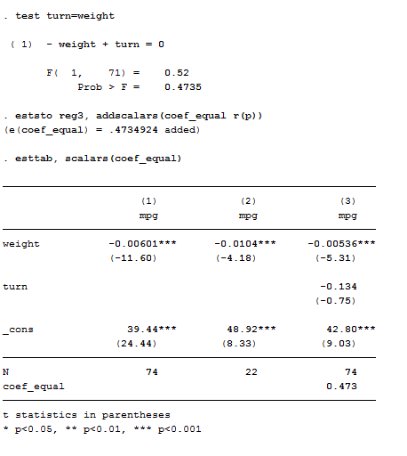
A very interesting option that eststo can do is save additional scalars for tabulation later like this:

qui reg mpg weight turn

test turn=weight

eststo reg3, addscalars(coef_equal r(p))

esttab, scalars(coef_equal)

Et voilà!

Remember that, if you want to add scalars to estimates, you can directly use the command estadd that is part of the -estout- package.

Three-way Tables: Never Limit Yourself

Stop wondering how to construct a three- or fourth-way table and learn how to do it. You can use three different strategies:

The first command you can use to construct a three-way table is tabulate. Its syntax works like that:

bysort var1: tab Var2 Var3 

The var1 is a categorical variable. For each level of it, you wish to see the cross tab of Var2 and Var3. You get a result showing the Frequency, row percentage and column percent because of the column row option. If you need to display different statistics just type help tabulate.

If you are dealing with survey data(we will discuss them later on) you must use a different command that uses the svy prefix, common to all survey-related tools -svy: prop-:

svy: prop var1, over(var2 var3)

The results list categories like _var1_1, _var1_2, but show a legend so that you know what is what. If prevalence is low, a lower confidence interval endpoint could fall below zero. In that case, you should use four instances of -svy: tab-, because -svy: tab- computes confidence intervals for the logit of a proportion, then transforms back. For Example:

svy, subpop(if var2==0 & var3==0) : Tab var1

The second and more comprehensive command that can help you out is table, which syntax is:

 table row_variable column_variable super_column_variable, by(super_row_var_list) contents(freq)

Finally, you can also install the tab3way package, which syntax is:

tab3way rowvar colvar supercolvar [weight] [if exp] [in range] [, cellpct rowpct colpct allpct rowtot coltot scoltot alltot format(%fmt) {freq|nofreq} usemiss]

It works with the by option and cross-tabulates three variables displaying any combination of cell frequencies, cell percents, row percents and column percents. “Missing” categories may be specified. It optionally provides row, column and supercolumn totals by temporarily augmenting observations in the existing data set and making a new category (labelled “TOTAL”) for each variable to accommodate these totals.

That’s all for now!  Stay tuned for new important insights!