When you deal with time series data, whatever data you have, this is ALL you have to know to handle it in Stata. At least, for now.

Good morning guys!

Today I am going to talk again about time series data but in a more practical and useful way. As I remembered you there, in order to work on time series, you first must tsset your data to advice Stata to recognize them.

Let’s open a proper dataset:

use http://www.stata-press.com/data/r12/wpi1.dta

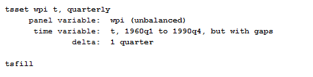
The first thing you have to control for, once you have tsset your data, is that there are no gaps in the time series (like a missing quarter or month). You can easily notice it, if this is the case in your data, because Stata will inform you that the time variable has gaps once you called the tsset command. How can you fix this? Use the command tsfill to fill in the gap in the time series.

..Then you can start play a bit!

Autocorrelation and Cross-Correlation

We can start by exploring autocorrelation and cross-correlation.

Autocorrelation

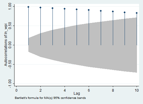
Autocorrelation represents the correlation between a variable and its previous values,  you can use the ac and pac commands to investigate it. ac produces a correlogram (a graph of autocorrelations) with pointwise confidence intervals that is based on Bartlett’s formula for MA(q) processes. In our case, it shows the correlation between the current value of the logarithmic transformation of wpi and its value ten lags ago. It can be used to define the q in MA(q) only in stationary series. pac produces a partial correlogram (a graph of partial autocorrelations) with confidence intervals calculated using a standard error of 1/sqrt(n). The residual variances for each lag may optionally be included on the graph. It shows also the correlation between the current value of the series and its value ten quarters ago, but without the effect of the nine previous lags. It can be used to define the p in AR(p) only in stationary series. So if you want you can type:

ac ln_wpi, lags(10)

And below you can find  the output you will obtain.. I personally dislike and find confusing this way to visualize autocorrelations.

If you agree with me, I suggest you to use the corrgram command that creates a table in which are shown both ac and pac, graphically and numerically. If you don’t want to see the graphs you can add the noplot options. If you want to reduce the number of lags displayed, the lags() option is what you need instead. In our example, I typed:

corrgram ln_wpi, lags(10)

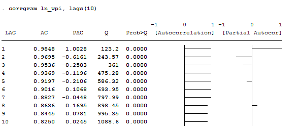
Apart for AC and PAC, this command displays the Box-Pierce’Q statistic, which tests the null hypothesis that all correlation up to lag k are equal to 0. This series shows significant autocorrelation given that the p-value is less than 0.05. therefore, we can reject the null that all lags are not autocorrelated. The graphic view of the AC shows a slow decay in the trend, suggesting non-stationarity. The graphic view of the PAC instead shows no spikes after the third lag, suggesting that all other lags are mirrors of the third one. Another easy way to see that the series is non-stationary is by plotting it.

twoway (tsline ln_wpi)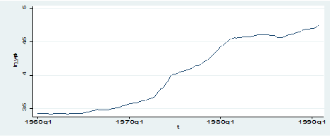

As we can observe, the series displays a clear increasing trend so it cannot be stationary at all.

Cross-correlation

If you want to explore the relationship between two time series, use the command xcorr, making sure that you always list the independent variable first and the dependent variable second. You can specify several options for this command that allow you to graphically visualize better the relationship. I, for example, typed:

xcorr ln_wpi wpi, lags(10) xlabel(-10(1)10,grid)

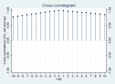
If you need to see the table, just put the table option instead of the xlabel() one. Of course, given that I only have one time series and its logarithmic transformation, the cross correlation is almost useless because, as we can expect, the relationship across the two is positive and reaches a peak in zero.

Lag Selection Criteria

There is something you cannot underestimate when using time series data that is the lag selection. Too many lags could indeed increase the error in the forecast whereas too few could leave out relevant information. There are some information criterion procedures to help come up with a proper selection of lags. The most commonly used are: Schwarz’s Bavesian info criteria (BIC), the Akaike’s information criteria (AIC) and the Hannan and Quin. The criterion is that you select the model with the smaller BIC or AIC. I usually trusted the BIC nore to choose the lag but there’s a useful command in Stata that allows you to plot them all in the same table and to freely choose among them.

In order to explore this issue, let’s use the following, more complete, dataset:

use http://www.stata-press.com/data/r11/lutkepohl2.dta

Now let’s use the varsoc command to see all the selection criterion procedures:

Varsoc ln_inc ln_consump, maxlag(10)

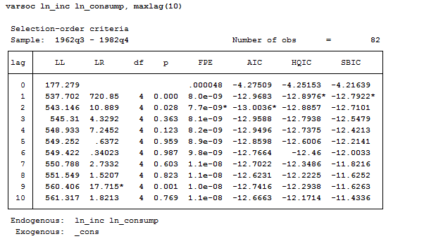
When the three criteria all agree, the selection is clear. But sometimes it can happen to get conflicting results. In this case, HQIC and SBIC suggest a lag of 2 whereas AIC a lag of 2. There are several papers on the argument so, if you need to be sure on what to believe, you are recommended to consult them.

Unit Root Test

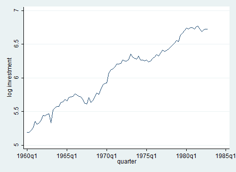
The most important thing to check with time series data is the presence of a unit root in the series.   In this section, we demonstrate how to evaluate if the series has a unit root. Having a unit root in a series means that there is more than one trend. Let’s look at logarithmic transformation of income across time and test for unit root.

line ln_inv qtr

One way to deal with unit roots is by using The Dickey-Fuller test, one of the most commonly used tests for stationarity. The null hypothesis is that the series has a unit root. The Stata command is:

dfuller ln_inv, lag(5)

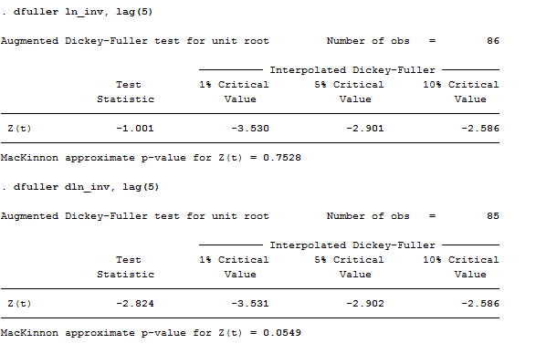
The test statistic shows that the investment series have a unit root, it lies within the acceptance region. One way to deal with stochastic trends (unit root) is by taking the first difference of the variable (second test above). In this case, we still fail to reject the null hypothesis! Panicked? Of course, not! If we reduce the lags from 5 to 2, you can see that the series has no more a unit root. Try to believe it!

If you are curious and you want to observe the associated regression when doing the Dickey-Fuller test, you can specify the regress option. Another useful one is trend, the trend option allows you to include a time trend term in the associated regression. In our case:

dfuller dln_inv, lag(2) trend regress 

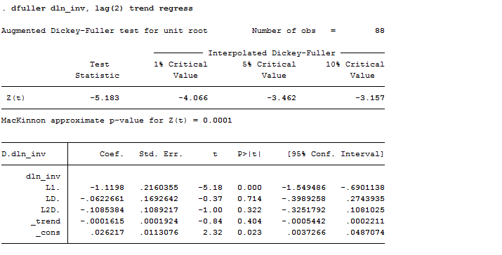
As you can observe, we can reject the hypothesis of a time trend in the series. Wait a second, how could it be possible? Well, remember that now we are working on the first differenced series of investments, which plot is no more the one above but this one:

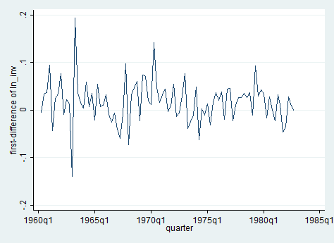
Does it make sense now? I hope so.

Useful tip: For panel data unit root tests, see Stata’s “xtunitroot” command.

Ok guys, for today it’s all. Next time we will run into AR, MA, ARIMA and VAR. Stay tuned!