All you have to know to use Panel Data proficiently using Stata
Good afternoon guys!
Today I want to spend some more words on Panel Data Analysis and extend our previous knowledge to what we know as Dynamic Panel data. When do we face those data? Well, let’s say that many economic issues are dynamic by nature, like employment models.
Usually, simple dynamic model regresses a dependent variable in polynomial in time or on lags of itself, so they are characterized by the presence of a lagged dependent variable among the regressors. To see what I am talking about, let’s write down an AR(1) model with individual specific effects:
![]()
In this case, we have reasons to suppose that our dependent variable is serially correlated over time through its lag (true state dependence), through some covariates, which may be serially correlated (observed heterogeneity), or through alpha (unobserved heterogeneity). If alphas are fixed-effects then the FE estimator is inconsistent. If we use the first differences to get rid of alphas, OLS estimates remain inconsistent because of the lagged variable. Arellano and Bond suggested to use first differences to get rid of alphas and then using an IV method. This proposed method leads to consistent but not necessarily efficient estimates and is a variation of OLS in first differences model that uses an unbalanced set of instruments with further lags as instruments. The moment conditions are formed assuming that particular levels of the dependent variable are orthogonal to the differenced disturbances.
Tip: This estimator works well on datasets with many panels and few periods (N>T) and it requires that there is no autocorrelation in the idiosyncratic errors.
The Stata command is xtabond, which basic syntax is:
xtabond y x
His constructor Arellano later revealed a potential weakness of this estimator because the lagged levels are often rather poor instruments for first-differenced variables. Therefore, a new estimator commonly termed system GMM was implemented to substitute this basic one (known as difference GMM). They both have one-step and two-step variants and the new command is now: xtabond2. The xtabond2 command offers you two opportunities. You can implement a difference GMM model that treats the model as a system of equations, one for each time period, that differ only in their instrument/moment condition sets. Alternatively, you may want to implement a system GMM model, the augmented version. This was created because lagged levels are often poor instruments for first differences, especially for variables that are close to a random walk. Thus, the original equations in levels can be added to the system, and the additional moment conditions could increase efficiency. In these equations, predetermined and endogenous variables in level are instrumented with suitable lags of their own first differences.
In order to work on a proper dataset we have to type in our Stata opened session the following command:
net from http://www.stata-press.com/data/imeus/
Here, a new window will open where you can install all the presented datasets. After you installed them all, you can select the one we need (traffic) by typing: use traffic.
This dataset is related to traffic accidents and we want to specify a model of fatal accidents as depending on the prior year’s value, the state’s spirits consumption and a time trend. We are going to use a set of instrument to control for endogeneity using the gmmstyle() option and use a variable as an IV instrument with the ivstyle() option. Then we can specify we want robust estimates the estimator to be in first differences with the noleveleq option. To review this command, you can estimate GMM-systems, GMM-levels and GMM-differences and you have both one- and two-step variants, with two-step estimates being asymptotically more efficient.
ssc install xtabond2
xtabond2 fatal L.fatal spircons year, gmmstyle(beertax spircons unrate perinc) ivstyle(year) twostep robust noleveleq
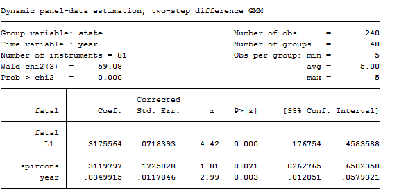
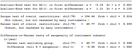
As we can see from the results, the Hansen test of over identifying restriction is satisfactory, as is the test for AR(2) errors.
Tip: Usually, we expect to reject the test for AR(1) errors in an Arellano-Bond model.
To compare the difference GMM estimator to the system GMM approach we are going to retype the same command, noleveleq option excluded:
xtabond2 fatal L.fatal spircons year, gmmstyle(beertax spircons unrate perinc) ivstyle(year) twostep robust
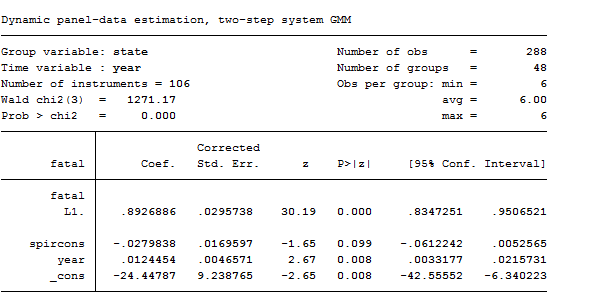
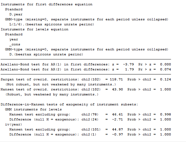
As you can see, contrasted with the previous model, this one works worse. Moreover, the marginally significant negative coefficient on spircons casts doubt on this specification. As the dynamic panel models are instrumental variables methods, it is particularly important to evaluate the Sargan-Hansen test results and the AR test for the autocorrelation of the residuals. By construction, the residuals of the differenced equation should possess serial correlation, but if the assumption of serial independence in the original errors is warranted, the differenced residuals should not exhibit significant AR(2) behavior. If a significant AR(2) statistic arises, the second lags of the endogenous variables are not appropriate instruments for their current values.
Finally, if you are confident that you can lose yourself in these models, there’s an updated version of this command that allows also for autocorrelated errors, xtdpd.
I want to know if I can use xtabond2 for macro panel (1983-2013) . Because I once tried it but sargan test was significant under first difference but very okay under step two. Please what can I do to eliminate this problem. Also I discovered that our vce(robust) under xtabond2 or xtdpdsys is different from other software because if you robust your result using the stata the result you will obtain is always different from others. Please help me out….
Dear Mr. Afolabi,
Thanks for having shared these thoughts with me.
Regarding your first doubt, I confirm you that xtabond2 can be used for macro panel. Indeed, xtabond2 works perfectly on panel data where the observations are more than the time period, as might be your case (N>T).
I would need more information regarding the model you used (instruments, variables, sample size) and the results of the test. What I can say now is:
1) Several studies of moment condition models have found that the Sargan test has poor size properties for samples of the size commonly encountered in econometric practice thus, I advise caution in the use of Sargan tests based on the full instrument set. A simple procedure (‘reducing lag’) is considered which often results in a Sargan test with good size and power properties in cases where T is large relative to N. Furthermore, Sargan tests based on a restricted instrument set can offer substantial gains in terms of power to detect serial correlation in the error term even when the test based on the full instrument set is correctly sized.
2) Arellano and Bover (1995) have developed a system GMM estimator, which combines the instruments of the first difference equation with additional instruments of the untransformed equation in level. Given the higher number of instruments, the system GMM estimator can lead to dramatic improvements in terms of efficiency as compared to the first difference GMM estimator. The validity of these additional instruments, which consist of past first difference values of the regressors, can again be tested through DIfference Sargan over-identification tests. You can try this method.
3) Regarding robust standard error… I was not aware of it!! I am really glad you discovered it. I will collect information and maybe write a small post about it.
I hope it helps,
Best Regards