Sometimes you have to deal with binary response variables. In this case, several OLS hypotheses fail and you have to rely on Logit and Probit.
Good afternoon Guys, I hope you are having a restful Sunday!
Today we will broadly discuss what you must know when you deal with binary response variable. Even though I don’t want to provide you a theoretical explanation I need to highlight this point.
OLS is known as a Linear Probability Model but, when it comes to binary response variable, it is not the best fit. Moreover, there are several problems when using the familiar linear regression line, which we can understand graphically.

As we can see, there are several problems with this approach. First, the regression line may lead to predictions outside the range of zero and one. Second, the functional form assumes the first observation of the explanatory variable has the same marginal effect on the dichotomous variable as the tenth, which is probably not appropriate. Third, a residuals plot would quickly reveal heteroskedasticity and a normality test would reveal absence of normality. Logit and Probit models solve each of these problems by fitting a nonlinear function to the data and are the best fit to model dichotomous dependent variable (e.g. yes/no, agree/disagree, like/dislike). The choice of Probit versus Logit depends largely on your preferences. Logit and Probit differ in how they define f(). The logit model uses something called the cumulative distribution function of the logistic distribution. The probit model uses something called the cumulative distribution function of the standard normal distribution to define f (). Both functions will take any number and rescale it to fall between 0 and 1. Hence, whatever α + βx equals; it can be transformed by the function to yield a predicted probability. If you are replicating a study, I suggest you to look through the literature on the topic and choose the most used model. Enough Theory for today!
In both model you can decide to include factor variables (i.e. Categorical ones) as a series of indicator variables by using i. Ready to start? Let’s take our friendly dataset, auto.dta. Don’t you remember the command? I introduced it there but we can revise it now: sysuse auto
Probit and Logit
Remember that Probit regression uses maximum likelihood estimation, which is an iterative procedure. In order to estimate a Probit model we must, of course, use the probit command. Nothing new under the sun.
probit foreign weight mpg i.rep78
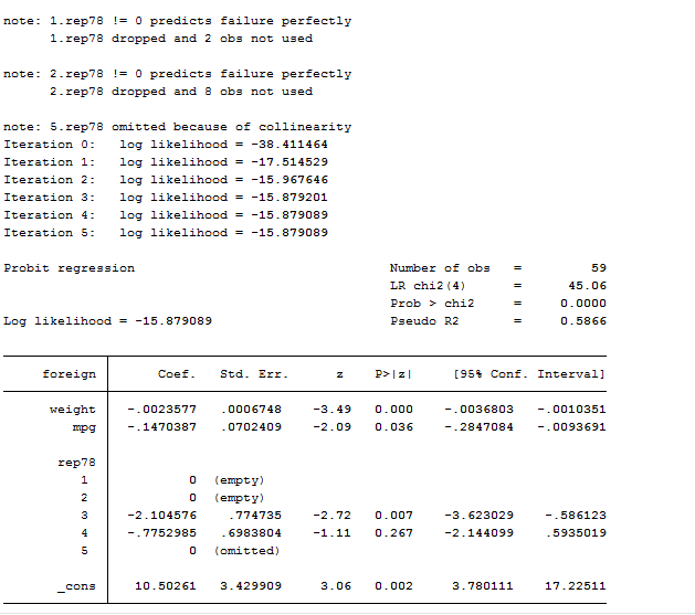
The above output is made by several element we never saw before, so we need to familiarize with them. The first one is the iteration log that indicates how quickly the model converges. The first iteration (called Iteration 0) is the log likelihood of the “null” or “empty” model; that is, a model with no predictors. At each iteration, the log likelihood increases because the goal is to maximize the log likelihood. When the difference between successive iterations is very small, the model is said to have “converged” and the iterating stops.
On the top right part, we can find the Likelihood Ratio Chi-Square Test (LR chi2) and its p-value. The number in the parentheses indicates the degrees of freedom of the distribution. Instead of R-squared we find the McFadden’s Pseudo R-Squared but this statistic is different from R-Squared and also its interpretation for the Probit model differs. The Probit regression coefficients give the change in the z-score for a one unit change in the predictor. I added a factor variable who was mainly dropped due to multicollinearity. As we already discussed in the post related to OLS regressions, there are several options available for this command like: vce(robust), noconstant, ect. If you missed the post, review it here.
After having performed the regression, we can proceed with post estimation results. We can test for an overall effect of rep78 using the test command. Below we see that the overall effect of rep78 is statistically insignificant.
test 3.rep78 4.rep78 // Joint probability that coefficients are all equal to zero
We can also test additional hypotheses about the differences in the coefficients for different levels of rep78. Below we test that the coefficient for rep78=3 is equal to the coefficient for rep78=4.
test 3.rep78 = 4.rep78
Another thing we can decide to do is to save the probit coefficients to a local macro:
local coef_probit = _b[x]
Then predict the probabilities from the probit after having called the regression command. predict is the command that gives you the predicted probabilities that the car type is foreign, separately for each observation in the sample, given the type’s regressor.
predict y_hat,pr
label var y_hat “Probit fitted values”
if you still believe there is a difference between computing a logit or a probit, then you have to try to regress this:
reg y_hatprobit y_hatlogit
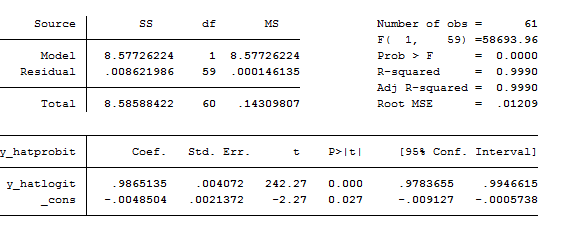
Look at the R-Squared. The models are practically equals. Feel free to switch between probit and logit whenever you want. The choice should not generally significantly affect your estimates.
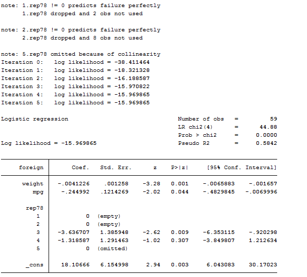
logit foreign weight mpg i.rep78
Logistic
There is almost no difference among logistic and logit models. The only thing that differs is that –logistic- directly reports coefficients in terms of odd ratio whereas if you want to obtain them from a logit model, you must add the or option. We can think about logit as a special case of the logistic equation. They both support the by() and if options and several others we have already reviewed.
Interpret Coefficients
When you use these models, you have to be careful in the interpretation of estimated coefficients. Indeed, you cannot just look at them and say that when weight increase by 1 the probability to have a foreign car decreases by an amount. If you want to declare such a thing, you must compute the fitted probabilities for specific values of the regressors. Moreover, you are not considering interaction terms in the model that might diminish or increase the effect of the weight covariate. Thus, it is important to find a way to compute the predicted probabilities for different possible individuals and to compare how those change when the value of a regressor changes. These are important features you have to take care of when dealing with dichotomous variables and related models. In order to explore coefficients’ interpretation, I am going to use an online database to explain you several differences among the margins, inteff and adjust commands. I am not going to discuss the mfx command because it was replaced by margins. If you still use this old command, please update your information by reading below. Indeed, several students and professionals of Stata are reluctant to use this command due to its syntax but it is extremely useful to investigate marginal effects and adjusted predictions. Let’s open a survey dataset oh health:
webuse nhanes2f
We want to study how the probability of become diabetic depends from, race and sex. I want to study if the effect of age is different depending of the sex so I am going to create the intersection variable:
gen femage=female*age
Then, I estimate a logistic regression, at first without this intersection:
logit diabetes black female age, nolog
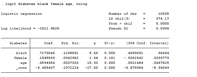
As we can observe, results show that getting older is bad for health but it seems to be unrelated with gender. The problem here is that we are not able to fully understand how bad it is to be old.
Adjust
That’s why we need to compute adjusted predictions that specify values for each regressor in the model and then compute the probability of the event occurring for an individual with those values. For, example we want to check which is the probability that an “average” 35 year old will have diabetes and compare it to the probability that an “average” 70 year old will. We need to type:
adjust age=35 black female, pr
adjust age=70 black female, pr
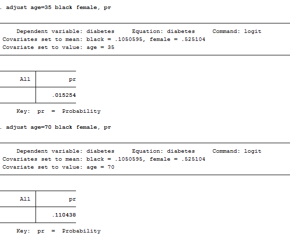
As we can observe, a 35 year old has less than 2 percent chance of having diabetes whereas a 70 year old has an 11 percent change. I used the expression “average” to indicate that I took mean values for the other independent variables in the model (female, black). However, this is an old command that is still on usage on Stata but it may be replaced easily by margins.
Margins
I should have obtained the same result by using the margin command. The –margin– command calculates predicted probabilities that are extremely useful to understand the model and was introduced in Stata 11. Margin looks at the discrete difference in probability between old and young for the different gender and race. Indeed, if we type:
margins, at(age=(35 70)) atmeans vsquish
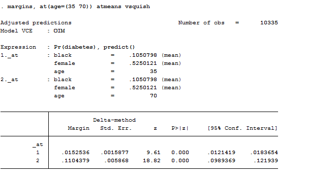
If we want to investigate the predicted probability of having diabetes at each age, holding all the other covariates at their means I could have also typed:
margins age, atmeans
There are several useful options of margin. The first one you can use is post that allows the results to be used with post-estimation command like test. Another one is predict, which allows you to obtain probabilities or linear predictions (i.e. predict(xb)). If we want to get the discrete difference in probability, we can use the dydx() option with the binary prediction. This option requests margins to report derivatives of the response with respect to the variable specified. Eyex() reports derivatives as elasticity. It finds the average partial effect of the explanatory variable on the probability observing a 1 in the dependent variable. This is taking the partial effects estimated by the logit for each observation then taking the average across all observations. This is extremely useful because the direct results of the logit estimations can not be directly interpreted as partial effects without a transformation.
If you have interaction effects in your model, you will need to specify your regressors using a particular notation Stata recognizes to be used to compute marginal effects:
- Creates dummy variable (as already mentioned here) // tells Stata variables are categorical (i.e. factor var)
- specifies continuous variables
# and ## specify interaction terms
Now we are going to study how margins deals with factor variables but first, let’s explain why adjust fails to compute them. If we type:
adjust age = 70 black female age2, pr
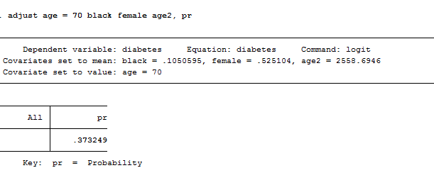
We can immediately notice that adjust reports a much higher predicted probability for an average individual of 70 years but it fails to control for the relationship between age and age2. Indeed, it uses the mean value of age2 in its calculations rather than the correct value of 70 squared. If we use margins with factor variables, the command recognized age and age2 to be not independent to each other and calculates accordingly. In fact:
logit diabetes i.black i.female age c.age#c.age, nolog
margins, at(age=70) atmeans
The smaller and correct estimate is not of 10.3 percent. Try to believe it. By doing this, Stata knows that if age=79 then age2=4900 and it hence computes the predicted values correctly. What about interaction terms?
if we want to study the interaction between age and female we have to regress:
logit diabetes black female age femage, nolog
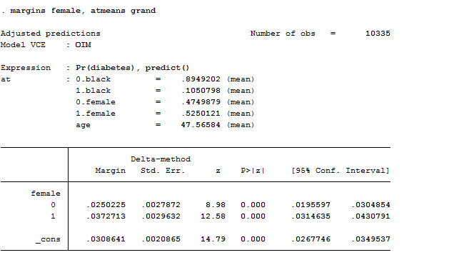
If we use adjust, we get wrong estimates because adjust does not recognize the relationship between female and femage thus it cannot understand that, if female=0, also femage will equal zero and it uses the average value instead. If you specify that your model has factor variables, margins recognizes that the different components of the interaction term are related and it computes correctly:
logit diabetes i.black i.female age i.female#c.age, nolog
margins female, atmeans grand
Marginal Effects
A partial or marginal effect measures the effect on the conditional mean of y of a change in one of the regressors. In the OLS it equals the slope coefficients. This is no longer the case in nonlinear models. Marginal effects for categorical variables shows how the probability of y=1 changes as the categorical variable changes from 0 to 1, after controlling for the other variables in the model. With a dichotomous independent variable like diabetes, the ME is the difference in the adjusted predictions for the two groups (diabetics & non-diabetics). Let’s see how to compute them:
logit diabetes i.black i.female age, nolog
margins, dydx(black female) atmeans
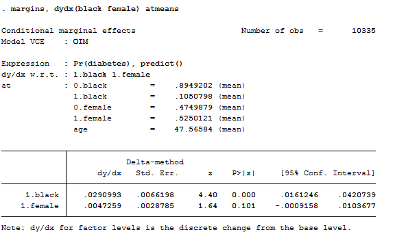
This result tells us that, if you have two otherwise-average individuals, one white and the other black, the black’s probability of having diabetes would be 2.9 percentage points higher.
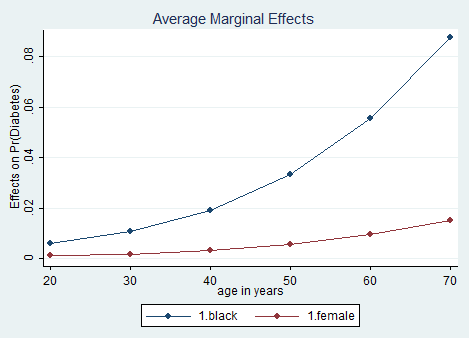
It can also be helpful to use graphs of predicted probabilities to understand and/or present the model. If we want to graph marginal effects for different ages in black people, we see that the effect of black differs greatly by age. How can we do that? Luckily, with the marginsplot command introduced in Stata 12.
margins, dydx(black female) at(age= (20 30 40 50 60 70)) vsquish
marginsplot, noci
The noci option tells Stata to not display the confidence intervals of the estimates. Other options related to graphs’ editor are available at my previous post on graphs and can be all used on marginsplot.
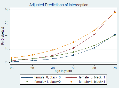
Let’s complicate our results a bit (Otherwise where is the fun?) by asking Stata to compute marginal effects for the intersection among race and gender. We must type:
logit diabetes i.black i.female age i.female#c.age, nolog
margins female#black, at(age=(20 30 40 50 60 70)) vsquish
marginsplot, noci title(Adjusted Predictions of Interception)
Inteff
There is another package to be installed in Stata that allows you to compute interaction effects, z-statistics and standard errors in nonlinear models like probit and logit models. The command is designed to be run immediately after fitting a logit or probit model and it is tricky because it has an order you must respect if you want it to work:
inteff depvar indepvar1 indepvar2 interaction_var1var2.
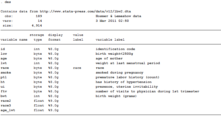
Indeed, it cannot contain less than four variables and the interacted variables cannot have higher order terms, such as squared terms. If the interaction term (at the fourth position) is a product of a continuous variable and a dummy variable, the first independent variable x1 has to be the continuous variable, and the second independent variable x2 has to be the dummy variable. The order of the second and third variables does not matter if both are continuous or both are dummy variables. Let’s make a practical example with two continuous variables interacted using a dataset named lbw2 but known as Hosmer & Lemeshow.
webuse lbw2
gen age_lwt=age*lwt
probit low age lwt age_lwt
inteff low age lwt age_lwt, savedata(C:\User\Michela\Stata\logit_inteff,replace) savegraph1(C:\User\Michela\Stata\figure1, replace) savegraph2(C:\User\Michela\Stata\figure2, replace)
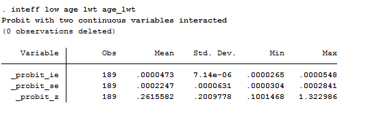
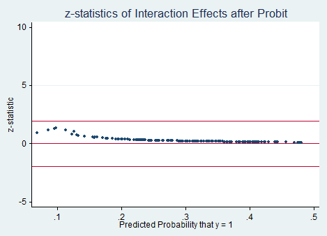
As you can see from the selected options you can choose to save both graphs produced and save the output. The saved file includes four variables that are the predicted probability, the interaction effect, the standard error and z-statistics of the interaction effect. You can also decide to save two scatter graphs that both predicted probabilities on the x-axis. The first graph plots two interaction effects against predicted probabilities, whereas the second one plots z-statistics of the interaction affect against predicted probabilities.
Fitstat
We may also wish to see measures of how well our model fits. This can be particularly useful when comparing competing models. The user-written command fitstat produces a variety of fit statistics as a post-estimation command but, if you want to use it, you need to install it first. In our example, this is what we get if we type the command after the probit regression.
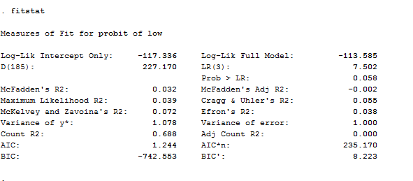
Here you have all you need to evaluate your model, starting from the AIC and BIC criteria. You don’t know what to do with them? I suggest you to check a good econometric book such as Wooldridge or Hamilton.
I think for now it is time to stop here. I leave to another time the study on how to create dynamic and multinomial logit and probit!
this is the best blog i have been wanting to see