Ready to play with your data? I assure you that it is simple and funny at the same time. Learn how to effectively manage them. 

Let’s start by opening the example dataset auto.dta that we already used here. There are several useful commands to outline the data, the observations or a single variable.

Manage your Data

The first command I suggest you to check if you want to manage your dataset  is describe

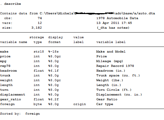
This command contains the description of the entire dataset, from variables to observations.

Storage type is the format in which those variables are recorded on Stata. Str18 indicates that the variable is defined as text or string(of length 18)  so, even if it contains numeric values, they are not recognized as numbers and thus cannot be inserted in regressions. This format is very important in survey data analysis because it usually represent the ID of the interviewed observations. If you want to obtain a numerical value from this variable you can transform it by using encode:

encode make, generates(model)

Now, from the string variable make I created a new numerical variable, model,  that is also useful if we want to declare data to be panel. This variable has now a different storage type that is long. This format, together with float, byte, double and  int, is the typical storage form that identifies a number.

Value labels  are labels for coded variables. In this case “Origin” may be coded 0 for Domestic and 1 for foreign cars. Variable labels are instead a description of what the variable represent and are usually composed of a few words. When you create a table of contents you can either specify if you want your variables names or labels to be displayed.

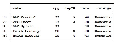
Another descriptive command useful to explore your data is  list. It shows the values of variables you want to control for. For example:

list make mpg rep78 turn foreign 

If you observe that your variables are not listed correctly, you can decide to set a criteria to analyze them. This is usually done with the sort command that arranges the observations of the data into ascending order based on the values of the specified variable. We can either type:

sort make

To obtain a listed data following the alphabetical order of make or:

bysort foreign: list

This command tells Stata to display car models divided by their domestic or foreign origin.

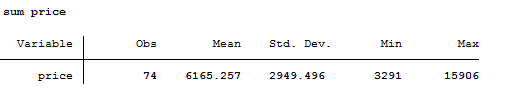
The last descriptive command is summarize. It provides a short resume of the variables’ statistics. We will extensively use it later on to construct Descriptive Statistics Tables.

sum price

NB. Stata recognizes a short version of its commands and imputes their output even if you do not write them in the long format (like sum, des, reg instead of summarize, describe, regress).

Manage your Variables

Now, you have learnt how to observe every component of your dataset. Don’t you like a name of one variable? Time to change it!

rename make Model

Rename intuitively works out by substituting the old name of the variable (make) with the new one (Model) you assigned it. You can also decide to rename an entire group of variables. If, for example, I have the variables year1 year2 and year3 I can decide to rename them as time1, time2 and time3 by typing:

rename year(#) time(#)

I suggest you to type help rename to see all the features available for this command if you have to perform other transformations.

Instead of variable’s names you can decide to change or add their labels. We already said that are commonly long sentences to explain which is the measure described. If you want to add a label or modify it just type:

label variable price “Price of the Car”

Whereas, if you want to change a value label, like the origin already defined for the variable foreign, you have to type:

 label define yesno 0 “no” 1 “yes”

label value foreign yesno

And, you will immediately see it in the Variables Window at the top right panel.

What if you want to create a new variable? Let’s say we want to construct the variable year1978 to remember that we have cross-sectional observations. The useful command is generate or gen:

gen year=1978

With this simple syntax I just created a vector cointainig the year of reference. Its derivation is a comprehensive command known as egen that  allows you to generate different variables containing the mean, the median or the standard deviation of a specified variable. It is also used to construct indexes, so, given its importance, I will dedicate an entire post to it. For now, let’s anticipate that its basic syntax is:

egen avg_price=mean(price)

Dummy Variables and Missing Data

Sometimes, using raw data as dependent variables is not that useful. In our dataset, for example, we can either use the prices as they are (and try to interpret how much a 1 mileage more on a model influence its price) or we can rather decide to create a new variable, a dummy, that takes a value of 1 if a certain criteria is met and a value of 0 otherwise. In order to construct this, we use two commands:

tab mpg, gen(dummy) 

This command is very intuitive but boring because it creates two mutually exclusive dummy variables, one for Foreign and the other for Domestic (so you have to delete one of the two). The other  simplest command ever is:

gen dummympg=0

replace dummympg=1 if mpg<=20

What did I just do? I told Stata to create a new variables that takes value of one if the mileage done by the car are less than 20, this could be also viewed as an indicator of conditions of use; we usually spend less for cars that were already used a lot. The problem here is that, constructing the variable like this, we are not taking into account any possible missing value. A useful command to check if there are missing values is codebook:

codebook mpg

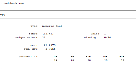
As we can see, this variable has no missing data. In case would have find some, another way to construct a variable is:

gen dummy_mpg=mpg>=20 if mpg<.

Here we told the software to consider missing values and to code them appropriately. Remember, the golden rule of missing data is: “If data are missing for less than 5% of your observations, is not such a big deal.” I will show you in another post all the ways to construct a dummy variable, for now, take this ones as granted. And remember to always check if your variables have missing data. How? Choose the right command!

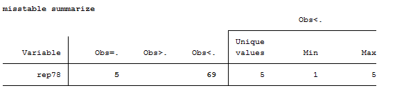
misstable summarize -> It gives an overview of missing values in the dataset. In our example, the variable rep78 contains missing values.

misstable patterns -> It shows the patterns in the data

mvencode _all, mv(999) -> Translate all the missing values from . to a default number 999

Thank God  for the Keep & Drop Commands

Preliminary Tip: Once launched, these commands are irreversible! I suggest you to save a copy of the file you have in memory with a different name before using them in order to avoid overwriting.

Then, you might wonder why you need to know them. Well, they are extremely helpful when you want to manage your data and get rid of all the redundant information. They work on variables and observations and you can play with them as much as you want.  Let’s say we only need to work on three variables, we can either type:

keep price make mpg

Or

drop rep78-foreign

The – sign means that you want to eliminate the entire list of variables between rep78 and foreign, bounds included. By doing so, our dataset is now made of three variables. Or maybe we want to analyze the subsample of economic cars, thus we type:

keep if price<=20

We can also decide that we want to get rid of outliers. How can we recognize if there is some in the distribution? Easy, just press tabulate, and you will see the table of frequencies of your variable.

tab mpg

Now that we discovered which are the lowest and highest values mpg can take, we can decide to cancel them:

keep if mpg>12 & mpg<41

If you are not fed up with these commands, you can also decide that you want to observe if there are missing values in your variable by typing:

tab rep78, missing 

Magic! We found the same result of the misstable summarize command. In all these cases, we reduced both the number of variables and the number of observations (=sample size) of this dataset. If you want to save your changes just type:

save newfile

After you cleaned and transformed raw data in something that has a logical sense, you are ready to combine data. Curious? Jump to the next post!

Summary: Describe – List – Sort – Summarize – Encode – Rename – Label – Gen – Egen – Tab – Codebook – Replace  Misstable Sum – Misstable pattern – Mvencode – Keep – Drop